Busulfan (Schreib 2024)
Source:vignettes/articles/Schreib_2024_busulfan.Rmd
Schreib_2024_busulfan.RmdModel and source
- Citation: Schreib KM, Braem DS, Zeilhofer UB, Mueller D, Guengoer T, Kraemer SD, Hauri-Hohl MM. Population Pharmacokinetic Modeling for Twice-Daily Intravenous Busulfan in a Large Cohort of Pediatric Patients Undergoing Hematopoietic Stem Cell Transplantation-A 10-Year Single-Center Experience. Pharmaceutics. 2024;16(1):13. doi:10.3390/pharmaceutics16010013. Author R code deposit (saemix objective function BuFunD.R and the time-dependence explainer kchange.R): https://gitlab.ethz.ch/skraemer/busulfan_2022.git
- Description: One-compartment population pharmacokinetic model with intravenous infusion and a time-varying elimination rate constant for busulfan in 124 pediatric patients undergoing hematopoietic stem cell transplantation (HSCT) at the University Children’s Hospital Zurich, October 2010 to February 2020, receiving twice-daily (q12h) 2-hour to 4-hour intravenous busulfan infusions as conditioning. Schreib 2024 fit ln(V) and ln(k) directly rather than CL and V, because ‘building the model on V and CL would result in two parameters with similar covariates … potentially masking the covariates for k’. Two further parameters describe an exponential decline of the elimination rate constant over the course of therapy: kel(t) = kel(0) * (1 + kel_exp_famp * (1 - exp(-kel_exp_kdes * t))), with kel_exp_famp = -0.167 (a 16.7% average fall in k and CL at steady state) and a 13.4 h half-life for the change. The fractional amplitude carries its own inter-individual variability and is doubled to -0.312 (a 31% fall) in the hemophagocytic lymphohistiocytosis / X-linked lymphoproliferative disease group. Volume scales near-proportionally with calculated total body water; the elimination rate constant depends on total body water, a postmenstrual-age maturation function, serum albumin, an acute lymphoblastic leukemia indicator, and the infusion duration. Total body water and the maturation function are derived inside model() from weight, height, age, and sex, so no separate columns are required. Because the elimination rate constant varies with time, the model must be integrated as an ODE: a closed-form linCmt() solution holds the elimination rate constant at its t = 0 value and therefore discards the time dependence that is the entire point of this paper. The error is large and one-sided: exposure per dosing interval is under-predicted by about 17% at steady state (45% in the HLH/XLP group). See the validation vignette for the demonstration.
- Article: https://doi.org/10.3390/pharmaceutics16010013
- Author R code deposit: https://gitlab.ethz.ch/skraemer/busulfan_2022.git
Schreib 2024 is a one-compartment intravenous-infusion population PK model for busulfan in children undergoing hematopoietic stem cell transplantation (HSCT). Two features make it unusual and are the focus of this validation:
-
It is parameterised on
ln(V)andln(k), notCLandV. The authors chose this deliberately: “Building the model on V and CL would result in two parameters with similar covariates … potentially masking the covariates for k and consequently fort1/2” (Section 3.2). Clearance is the derived quantityCL = k * V. -
The elimination rate constant declines over the course of
therapy. Two extra parameters describe an exponential
relaxation of
kfrom its value at the first dose toward a lower asymptote, with a 13.4 h half-life. The amplitude of that decline carries its own inter-individual variability and is roughly doubled in the HLH/XLP diagnosis group.
Population
The model was built on 124 consecutive patients transplanted at the University Children’s Hospital Zurich between October 2010 and February 2020 (Table 1 of Schreib 2024). Median age was 4.3 years (range 0.2-27.0); 23 patients (18%) were under 1 year and 118 (95%) were under 18. Median body weight was 17.2 kg (range 4.3-85.0) and median body surface area 0.71 m2 (range 0.25-2.06). 35 of 124 patients (28%) were female. 42 patients (34%) were transplanted for malignant disease – including 13 (10%) with acute lymphoblastic leukemia – and 82 (66%) for non-malignant disease, including 14 (11%) with hemophagocytic lymphohistiocytosis or X-linked lymphoproliferative disease.
Busulfan was given twice daily as an intravenous infusion over four hours (October 2010 to September 2014) or three hours (October 2014 onward), for four to ten doses over two to five days. The initial dose targeted a single-interval AUC of 9-12 mgh/L. Patients with non-malignant disease other than metabolic disease received reduced-intensity conditioning targeting a cumulative AUC of 45-70 mgh/L; patients with malignant or metabolic disease received myeloablative conditioning targeting 80-100 mg*h/L (Section 2.2). In total 2376 plasma concentrations from 373 infusions were analysed, with no data excluded.
The same information is available programmatically via
readModelDb("Schreib_2024_busulfan")()$population.
Source trace
Every ini() entry in
inst/modeldb/specificDrugs/Schreib_2024_busulfan.R carries
an in-file comment naming its origin. They are collected here for
review.
| Equation / parameter | Value | Source location |
|---|---|---|
lvc |
2.459 | Table 3, theta_V1 (SE 0.0189); untransformed 11.70
L |
e_tbw_vc |
0.931 | Table 3, theta_V2 (SE 0.0233, p < 0.001) |
e_tinf_vc |
0.226 | Table 3, theta_V3 (SE 0.0356, p < 0.001) |
lkel |
-1.007 | Table 3, theta_k1 (SE 0.0329); untransformed 0.365
1/h |
e_tbw_kel |
-0.189 | Table 3, theta_k2 (SE 0.0411, p < 0.001) |
e_fmat_kel |
0.697 | Table 3, theta_k3 (SE 0.2001, p < 0.001) |
e_alb_kel |
0.331 | Table 3, theta_k4 (SE 0.1073, p = 0.001) |
e_all_kel |
-0.210 | Table 3, theta_k5 (SE 0.0592, p < 0.001) |
e_tinf_kel |
-0.161 | Table 3, theta_k6 (SE 0.0420, p < 0.001) |
kel_exp_famp |
-0.167 | Table 3, theta_dk1 (SE 0.0191) |
e_hlhxlp_kel_exp_famp |
-0.145 | Table 3, theta_dk2 (SE 0.0540, p = 0.0035) |
lkel_exp_kdes |
-2.965 | Table 3, theta_kappa_k (SE 0.1094); untransformed
0.0516 1/h |
etalvc |
0.029 | Table 3, IIV block, Omega^2 of ln(V) (Omega 0.169, shrinkage 5.5%) |
etalkel |
0.033 | Table 3, IIV block, Omega^2 of ln(k) (Omega 0.182, shrinkage 12.5%) |
etakel_exp_famp |
0.032 | Table 3, IIV block, Omega^2 of dk (Omega 0.180, shrinkage 12.5%) |
addSd |
0.076 | Table 3, residual error (SE 0.0008); additive error model per Sections 2.5 and 3.3 |
d/dt(central) <- -kel_exp_total * central |
n/a | Equation (1) (one-compartment infusion superposition) |
kel_exp_total (time dependence of k) |
n/a | Equation (2); see “Which time-varying k?” below |
tbw (total body water) |
n/a | Equation (7), after Wells 2005 |
fmat (maturation function) |
n/a | Equation (9), after Hassine 2021; PMA = postnatal age + 40 weeks (Section 2.7) |
| Reference values (TBW 10 L, Alb 30 g/L, Tinf 3 h, Fmat 1) | n/a | Table 3, “Reference value” column |
Which time-varying k? Equation (2), not Equation
(3)
Schreib 2024 prints two different time-varying rate constants, and only one of them is the model:
-
Equation (2),
k*(t) = k * (1 + dk * (1 - exp(-kappa_k * t)))– the instantaneous rate constant. -
Equation (3),
k'(t)– the running time-average ofk*(t), obtained by integrating it. This exists only because the authors fit insaemixwith a closed-form superposition likelihood and no ODE solver, so the per-interval exponential needed an interval-averaged rate constant.
They are materially different: k*/k = 0.881 versus
k'/k = 0.929 at 24 h, a roughly 5% difference in AUC. The
packaged model uses Equation (2), because an ODE integrates the
instantaneous rate constant directly. Two independent lines of evidence
confirm that this, and not Equation (3), is the published model:
- The authors’ deposited script
kchange.Rbuilds the concentration profile by stepwise integration ofk*(t)and labels that construction “this is the reference”;k'appears there as one of three approximations tested against it. - Figure 4B plots simulated
CL(t)normalised toCL(t = 0). Normalising cancels every covariate and every unit, so the curve reads out the time dependence alone. The check is reproduced numerically below.
The chunk below is the falsification, not decoration: if the packaged model had encoded Equation (3), the “Eq (2)” column would not match the values read off Figure 4B, and the HLH/XLP subgroup line would miss by about 0.09.
kappa <- exp(-2.965)
eq2 <- function(t, dk) 1 + dk * (1 - exp(-kappa * t))
eq3 <- function(t, dk) {
  (((1 + dk) * t - dk / kappa - ((eq2(t, dk)) - (1 + dk)) / kappa) / t)
}
tibble::tibble(
  `Time (h)`               = c(24, 48, 60),
  `Fig 4B mean (read off)` = c(0.87, 0.84, 0.837),
  `Eq (2), dk = -0.167`    = round(eq2(c(24, 48, 60), -0.167), 3),
  `Eq (3), dk = -0.167`    = round(eq3(c(24, 48, 60), -0.167), 3),
  `Fig 4B HLH/XLP (read off)` = c(0.775, 0.72, 0.70),
  `Eq (2), dk = -0.312`    = round(eq2(c(24, 48, 60), -0.312), 3),
  `Eq (3), dk = -0.312`    = round(eq3(c(24, 48, 60), -0.312), 3)
) |>
  knitr::kable(
    caption = paste(
      "Figure 4B of Schreib 2024 discriminates the two printed time-varying",
      "rate constants. Equation (2) matches both the population line and the",
      "HLH/XLP line; Equation (3) matches neither."
    )
)| Time (h) | Fig 4B mean (read off) | Eq (2), dk = -0.167 | Eq (3), dk = -0.167 | Fig 4B HLH/XLP (read off) | Eq (2), dk = -0.312 | Eq (3), dk = -0.312 |
|---|---|---|---|---|---|---|
| 24 | 0.870 | 0.881 | 0.929 | 0.775 | 0.779 | 0.867 |
| 48 | 0.840 | 0.847 | 0.895 | 0.720 | 0.714 | 0.803 |
| 60 | 0.837 | 0.841 | 0.885 | 0.700 | 0.702 | 0.784 |
Time-varying clearance and the linCmt() conversion
Every rxSolve() call in this vignette passes
useLinCmt = FALSE. That is now belt and braces
rather than a necessity, and it is kept deliberately – see below.
Schreib 2024 is a one-compartment model with linear elimination,
which is the structure rxSolve() recognises and can rewrite
into a closed-form linCmt() solution. That closed form can
only carry a constant elimination rate constant, so
through rxode2 5.1.6 the rewrite silently substituted kel
at t = 0 for all time and discarded the entire time
dependence – the whole subject of this paper. The failure was silent,
one-sided and large: under the default flag every interval collapsed to
exactly Dose / (kel(0) * vc).
rxode2 5.1.7 closed that hole from the other side. It now refuses the
ODE-to-linCmt() conversion when the conversion would change
a rate or when the model carries an exogenous input term, which covers
this model, so the rewrite no longer happens and both flags give the
same answer. The check below solves the same regimen both ways and
asserts exactly that: the time dependence survives, and the two paths
agree.
Passing the flag explicitly is still worth doing. It states which
solver path the numbers came from instead of inheriting a package
default – and that default itself changed in rxode2 5.1.8, from
TRUE to FALSE.
# rxode2() turns the model function returned by readModelDb() into the rxUi
# object that zeroRe() and rxSolve() operate on.
mod <- rxode2::rxode2(readModelDb("Schreib_2024_busulfan"))
trap_ev <- rxode2::et(amt = 40, dur = 3, cmt = "central", ii = 12, addl = 7) |>
  rxode2::et(seq(0, 96, by = 0.25), cmt = "central") |>
  as.data.frame() |>
  dplyr::mutate(WT = 16.5, HT = 101.2, AGE = 4.3, SEXF = 0,
                ALB = 30, TINF = 3, DIS_ALL = 0, DIS_HLHXLP = 0)

interval_auc_of <- function(s) {
  vapply(1:8, function(i) {
    seg <- s[s$time >= 12 * (i - 1) & s$time <= 12 * i, ]
    sum(diff(seg$time) * (utils::head(seg$Cc, -1) + utils::tail(seg$Cc, -1)) / 2)
  }, numeric(1))
}

trap_default <- interval_auc_of(
  rxode2::rxSolve(rxode2::zeroRe(mod), trap_ev, returnType = "data.frame",
                  omega = NA, useLinCmt = TRUE))
trap_ode <- interval_auc_of(
  rxode2::rxSolve(rxode2::zeroRe(mod), trap_ev, returnType = "data.frame",
                  omega = NA, useLinCmt = FALSE))

tibble::tibble(
  `Dosing interval`             = 1:8,
  `AUC, useLinCmt = TRUE`       = round(trap_default, 3),
  `AUC, useLinCmt = FALSE`      = round(trap_ode, 3),
  `Difference`                  = sprintf("%.1f%%", 100 * (trap_default / trap_ode - 1))
) |>
  knitr::kable(
    caption = paste(
      "From rxode2 5.1.7 the ODE-to-linCmt conversion is refused for this",
      "model, so both columns rise as clearance falls and the under-prediction",
      "is zero. Before 5.1.7 the converted column did not move after the first",
      "interval, holding kel at its t = 0 value."
    )
)| Dosing interval | AUC, useLinCmt = TRUE | AUC, useLinCmt = FALSE | Difference |
|---|---|---|---|
| 1 | 9.507 | 9.507 | 0.0% |
| 2 | 10.393 | 10.393 | 0.0% |
| 3 | 10.826 | 10.826 | 0.0% |
| 4 | 11.075 | 11.075 | 0.0% |
| 5 | 11.216 | 11.216 | 0.0% |
| 6 | 11.293 | 11.293 | 0.0% |
| 7 | 11.335 | 11.335 | 0.0% |
| 8 | 11.358 | 11.358 | 0.0% |
# Regression guard, in two parts. The first is the physics and has always held:
# clearance falls with time, so interval AUC must rise. The second used to
# assert the linCmt column was FLAT -- the defect. rxode2 5.1.7 refuses the
# conversion for this model, so the two paths now agree instead, and asserting
# that catches both a reintroduced rewrite and a silent divergence.
stopifnot(trap_ode[8] / trap_ode[1] > 1.15,
          max(abs(trap_default / trap_ode - 1)) < 1e-6)
Typical values at the reference covariates
Table 3 reports the back-transformed typical values at its own
reference covariates (TBW 10 L, Fmat 1, albumin 30 g/L, no
ALL, infusion 3 h): V = 11.70 L and
k = 0.365 1/h. The packaged model must reproduce both
exactly. Fmat reaches 1 only asymptotically, so the check
is run at the covariate values the reference row describes rather than
at any particular age.
# Weight / height that give TBW = exactly 10 L for a male at the cohort median
# age of 4.3 years, using Equation (7). Height follows the cohort's own
# weight-BSA relation (see the virtual-cohort section).
tbw_of <- function(w, h, age, sexf) {
  exp(-2.952 + 0.551 * log(w) + 0.796 * log(h) + 0.008 * age - 0.047 * sexf)
}
ht_of  <- function(w) (0.71 * (w / 17.2)^(2 / 3))^2 * 3600 / w
ref_wt <- stats::uniroot(function(w) tbw_of(w, ht_of(w), 4.3, 0) - 10,
                         c(5, 40))$root
ref_ht <- ht_of(ref_wt)

ref_ev <- rxode2::et(amt = 40, dur = 3, cmt = "central") |>
  rxode2::et(c(0, 0.5, 1, 2, 3, 4, 6, 9, 12), cmt = "central") |>
  as.data.frame() |>
  dplyr::mutate(WT = ref_wt, HT = ref_ht, AGE = 4.3, SEXF = 0,
                ALB = 30, TINF = 3, DIS_ALL = 0, DIS_HLHXLP = 0)

ref_sim <- rxode2::rxSolve(rxode2::zeroRe(mod), ref_ev, returnType = "data.frame",
                           omega = NA, useLinCmt = FALSE)

# Fmat at the cohort median age, used to lift kel back to its Fmat = 1 reference
fmat_ref <- 1 / (1 + ((52 * 4.3 + 40) / 46)^(-2.3))

tibble::tibble(
  Quantity  = c("V at reference covariates (L)",
                "k at reference covariates (1/h)",
                "kappa_k (1/h)",
                "Half-life of the change in k (h)"),
  Model     = c(ref_sim$vc[1],
                ref_sim$kel_exp_total[ref_sim$time == 0][1] / fmat_ref^0.697,
                exp(-2.965),
                log(2) / exp(-2.965)),
  Published = c(11.70, 0.365, 0.0516, 13.4),
  Source    = c("Table 3, untransformed theta_V1",
                "Table 3, untransformed theta_k1",
                "Table 3, untransformed theta_kappa_k",
                "Section 3.4 text")
) |>
  dplyr::mutate(Model = round(Model, 4)) |>
knitr::kable(caption = "Typical values reproduced from the packaged model.")| Quantity | Model | Published | Source |
|---|---|---|---|
| V at reference covariates (L) | 11.6931 | 11.7000 | Table 3, untransformed theta_V1 |
| k at reference covariates (1/h) | 0.3653 | 0.3650 | Table 3, untransformed theta_k1 |
| kappa_k (1/h) | 0.0516 | 0.0516 | Table 3, untransformed theta_kappa_k |
| Half-life of the change in k (h) | 13.4434 | 13.4000 | Section 3.4 text |
Published covariate-effect statements
Schreib 2024 states several covariate effects in words in Section 3.2. Each is a closed-form consequence of Table 3 and can be checked exactly.
tibble::tribble(
  ~Statement, ~Computed, ~Published,
  "Doubling TBW reduces k (factor 2^-0.189)",
    sprintf("%.1f%% reduction", 100 * (1 - 2^-0.189)),                "12%",
  "ALL reduces k (factor exp(-0.210))",
    sprintf("%.1f%% reduction", 100 * (1 - exp(-0.210))),             "20% on average",
  "Steady-state fall in k and CL (dk = -0.167)",
    sprintf("%.1f%% reduction", 100 * 0.167),                         "16.7%",
  "Fall in k and CL for HLH/XLP (dk = -0.167 - 0.145)",
    sprintf("%.1f%% reduction", 100 * 0.312),                         "31%",
  "Fmat at 98 weeks postmenstrual age",
    sprintf("%.3f", 1 / (1 + (98 / 46)^(-2.3))),                      "0.85",
  "Fmat at 46 weeks postmenstrual age",
    sprintf("%.3f", 1 / (1 + (46 / 46)^(-2.3))),                      "0.5",
  "CL = k * V ratio for a 4 h vs a 3 h infusion",
    sprintf("%.3f", exp(0.226 - 0.161)),                              "virtually independent of Tinf"
) |>
  knitr::kable(
    caption = paste(
      "Covariate-effect statements in Section 3.2 of Schreib 2024, recomputed",
      "from the Table 3 estimates. The paper's ALL sentence prints the factor",
      "as 100 * (1 - 10^-0.21), which is a typographical error for the natural",
      "base; 10^-0.21 would be a 38% reduction, not the 20% the sentence claims."
    )
)| Statement | Computed | Published |
|---|---|---|
| Doubling TBW reduces k (factor 2^-0.189) | 12.3% reduction | 12% |
| ALL reduces k (factor exp(-0.210)) | 18.9% reduction | 20% on average |
| Steady-state fall in k and CL (dk = -0.167) | 16.7% reduction | 16.7% |
| Fall in k and CL for HLH/XLP (dk = -0.167 - 0.145) | 31.2% reduction | 31% |
| Fmat at 98 weeks postmenstrual age | 0.851 | 0.85 |
| Fmat at 46 weeks postmenstrual age | 0.500 | 0.5 |
| CL = k * V ratio for a 4 h vs a 3 h infusion | 1.067 | virtually independent of Tinf |
The infusion-duration row is the one place where “virtually” is doing real work: the two opposite-signed effects do not cancel exactly, leaving clearance about 6.7% higher for a 4 h than for a 3 h infusion. The paper’s claim is qualitative and the model reproduces the near-cancellation it describes.
Virtual cohort
Original patient data are confidential and are explicitly not included in the authors’ deposit (“The patient data are not available here as they are confidential”). The cohort below is virtual, with covariate distributions built to match the Table 1 marginals.
Body size is generated from a single weight variable. Body surface
area follows BSA = 0.71 * (WT / 17.2)^(2/3), anchored on
the cohort median (17.2 kg, 0.71 m2); this relation
independently reproduces both reported BSA extremes –
it gives 0.28 m2 at the 4.3 kg minimum and 2.06 m2
at the 85 kg maximum, against Table 1’s reported range of 0.25-2.06
m2. Height is then recovered by inverting the Mosteller
relation (Equation 6), HT = BSA^2 * 3600 / WT, exactly as
the authors’ BuSaemix.R does.
set.seed(20240113)

# Arm sizes follow the Table 1 indication split: 42 malignant + 8 metabolic of
# 124 (40%) received myeloablative conditioning, the remaining 74 (60%) reduced
# intensity. Keeping that split is what makes the within-arm disease
# prevalences reproduce the whole-cohort 10% ALL and 11% HLH/XLP.
n_mac <- 80L
n_ric <- 120L

# Median weight-for-age anchors spanning the Table 1 age range. Interpolated on
# the log-log scale, so the curve is smooth and monotone. This is an assumption
# (see "Assumptions and deviations"); it is calibrated to pass through the
# cohort median of 17.2 kg at 4.3 years.
wt_anchor_age <- c(0.2, 1, 2, 4.3, 10, 14, 18, 27)
wt_anchor_wt  <- c(5.0, 9.5, 12.5, 17.2, 32, 48, 60, 70)
median_wt_for_age <- function(age) {
  exp(stats::approx(log(wt_anchor_age), log(wt_anchor_wt),
                    xout = log(age), rule = 2)$y)
}

# Age is drawn from the three bands Table 1 tabulates (18% under 1 year, 77%
# between 1 and 18, 5% over 18) rather than from a single lognormal, because a
# single lognormal matching the 4.3-year median generates only ~6% infants and
# would barely exercise the Fmat maturation term.
sample_age <- function(n) {
  band <- sample(c("infant", "child", "adult"), n, replace = TRUE,
                 prob = c(0.18, 0.77, 0.05))
  ifelse(
    band == "infant", exp(stats::runif(n, log(0.2), log(1))),
    ifelse(band == "adult", stats::runif(n, 18, 27),
           pmin(pmax(exp(stats::rnorm(n, log(5.0), 0.75)), 1), 18))
  )
}

# Exact counts rather than rbinom draws, so the reported prevalences are the
# Table 1 targets and not a binomial sample around them.
exact_flag <- function(n, p) as.integer(seq_len(n) %in% sample.int(n, round(p * n)))

make_cohort <- function(n, conditioning, n_doses, id_offset = 0L) {
  age <- sample_age(n)
  wt  <- median_wt_for_age(age) * exp(stats::rnorm(n, 0, 0.22))
  wt  <- pmin(pmax(wt, 4.3), 85)
  bsa <- 0.71 * (wt / 17.2)^(2 / 3)
  ht  <- bsa^2 * 3600 / wt
  # Albumin: lognormal about the 30 g/L reference, scaled so ~95% of subjects
  # fall inside the Table 3 population range of ln(Alb/30) (-0.45 to 0.48).
  alb <- 30 * exp(stats::rnorm(n, 0, 0.16))
  tibble::tibble(
    id           = id_offset + seq_len(n),
    AGE          = age,
    WT           = wt,
    HT           = ht,
    SEXF         = exact_flag(n, 0.28),
    ALB          = alb,
    # 3 h from Oct 2014, 4 h before; the cohort spans both protocols.
    TINF         = ifelse(exact_flag(n, 0.5) == 1, 3, 4),
    # 13 of the 50 myeloablative patients had ALL (26%); 14 of the 74
    # reduced-intensity patients had HLH/XLP (19%).
    DIS_ALL      = if (conditioning == "MAC") exact_flag(n, 0.26) else 0L,
    DIS_HLHXLP   = if (conditioning == "RIC") exact_flag(n, 0.19) else 0L,
    conditioning = conditioning,
    n_doses      = n_doses
  )
}

# Malignant and metabolic disease -> myeloablative (MAC, cAUC 80-100 mg*h/L,
# 8 doses); other non-malignant disease -> reduced intensity (RIC, cAUC
# 45-70 mg*h/L, 6 doses).
subjects <- dplyr::bind_rows(
  make_cohort(n_mac, "MAC", 8L, id_offset = 0L),
  make_cohort(n_ric, "RIC", 6L, id_offset = n_mac)
)

# Expand each subject into q12h infusion doses plus a 0.25 h observation grid.
build_events <- function(subjects, doses) {
  dose_rows <- subjects |>
    dplyr::left_join(doses, by = "id") |>
    tidyr::uncount(n_doses, .id = "dose_no") |>
    dplyr::mutate(
      time = 12 * (dose_no - 1),
      evid = 1L, cmt = "central", dur = TINF
    ) |>
    dplyr::select(-dose_no)
  obs_rows <- subjects |>
    dplyr::left_join(doses, by = "id") |>
    tidyr::crossing(time = seq(0, 96, by = 0.25)) |>
    dplyr::filter(time <= 12 * n_doses) |>
    dplyr::mutate(amt = NA_real_, evid = 0L, cmt = "central", dur = NA_real_)
  dplyr::bind_rows(dose_rows, obs_rows) |>
    dplyr::arrange(id, time, dplyr::desc(evid))
}

# Step 1: solve a typical-value profile at a reference 100 mg dose to obtain
# each subject's first-interval AUC, then scale the dose to the paper's 9-12
# mg*h/L per-interval target (midpoint 10.5). This is model-informed dosing
# using population parameters only -- the individual random effects are not
# known to the prescriber, so zeroRe() is the right basis for the dose.
probe_ev <- build_events(subjects, tibble::tibble(id = subjects$id, amt = 100))
probe <- rxode2::rxSolve(rxode2::zeroRe(mod), probe_ev, omega = NA,
                         keep = c("conditioning"), returnType = "data.frame",
                         useLinCmt = FALSE)
#> Warning: multi-subject simulation without without 'omega'

auc_first <- probe |>
  # rxSolve returns observation rows only, so there is no evid column here.
  dplyr::filter(time <= 12) |>
  dplyr::group_by(id) |>
  dplyr::summarise(
    auc1 = sum(diff(time) * (head(Cc, -1) + tail(Cc, -1)) / 2),
    .groups = "drop"
  )

doses <- auc_first |>
  dplyr::mutate(amt = round(100 * 10.5 / auc1, 1)) |>
  dplyr::select(id, amt)

events <- build_events(subjects, doses)
stopifnot(!anyDuplicated(unique(events[, c("id", "time", "evid")])))
subjects |>
  dplyr::left_join(doses, by = "id") |>
  dplyr::group_by(conditioning) |>
  dplyr::summarise(
    n = dplyr::n(),
    `Age median (y)`  = round(stats::median(AGE), 1),
    `Weight median (kg)` = round(stats::median(WT), 1),
    `BSA median (m2)` = round(stats::median(0.71 * (WT / 17.2)^(2 / 3)), 2),
    `Female (%)` = round(100 * mean(SEXF)),
    `Dose median (mg)` = round(stats::median(amt), 1),
    .groups = "drop"
  ) |>
  dplyr::rename(Conditioning = conditioning, N = n) |>
  knitr::kable(
    caption = paste(
      "Virtual cohort. Cohort-wide medians for age (4.3 y), weight (17.2 kg)",
      "and BSA (0.71 m2) target Table 1 of Schreib 2024."
    )
)| Conditioning | N | Age median (y) | Weight median (kg) | BSA median (m2) | Female (%) | Dose median (mg) |
|---|---|---|---|---|---|---|
| MAC | 80 | 4.3 | 16.5 | 0.69 | 28 | 42.8 |
| RIC | 120 | 4.4 | 17.3 | 0.71 | 28 | 46.9 |
Simulation
sim <- rxode2::rxSolve(
  mod, events = events,
  keep = c("conditioning", "DIS_ALL", "DIS_HLHXLP", "TINF", "WT"),
  returnType = "data.frame",
  useLinCmt = FALSE
)
stopifnot(dplyr::n_distinct(sim$id) == nrow(subjects))
Replicate published figures
Figure 4B – simulated CL(t) normalised to CL(t = 0)
Figure 4B of Schreib 2024 shows simulated
CL(t)/CL(t = 0) with a solid line from the population fixed
effects, a broken line for the HLH/XLP diagnosis group, and shaded 80%
and 95% prediction bands. Because volume is time-invariant in this
model, CL(t)/CL(0) is identical to k(t)/k(0),
which is what the packaged model exposes as
kel_exp_total.
# Replicates Figure 4B of Schreib 2024.
cl_rel <- sim |>
  dplyr::group_by(id) |>
  dplyr::mutate(rel = kel_exp_total / dplyr::first(kel_exp_total)) |>
  dplyr::ungroup()

bands <- cl_rel |>
  dplyr::group_by(time) |>
  dplyr::summarise(
    lo95 = stats::quantile(rel, 0.025), lo80 = stats::quantile(rel, 0.10),
    hi80 = stats::quantile(rel, 0.90),  hi95 = stats::quantile(rel, 0.975),
    .groups = "drop"
  )

typical <- tibble::tibble(time = seq(0, 96, by = 0.5)) |>
  dplyr::mutate(
    `Population fixed effects` = eq2(time, -0.167),
    `HLH/XLP fixed effects`    = eq2(time, -0.312)
  ) |>
  tidyr::pivot_longer(-time, names_to = "Line", values_to = "rel")

ggplot() +
  geom_ribbon(data = bands, aes(time, ymin = lo95, ymax = hi95),
              fill = "grey80") +
  geom_ribbon(data = bands, aes(time, ymin = lo80, ymax = hi80),
              fill = "grey60") +
  geom_line(data = typical, aes(time, rel, linetype = Line), linewidth = 0.8) +
  geom_hline(yintercept = 1, linetype = "dotted") +
  geom_vline(xintercept = c(24, 48), linetype = "dotted") +
  scale_x_continuous(breaks = seq(0, 96, 12)) +
  labs(x = "Time (h)", y = "CL(t) / CL(t = 0)", linetype = NULL,
       title = "Figure 4B - simulated CL(t) normalised to the start of therapy",
       caption = "Replicates Figure 4B of Schreib 2024. Dotted verticals at 24 and 48 h.") +
  theme(legend.position = "bottom")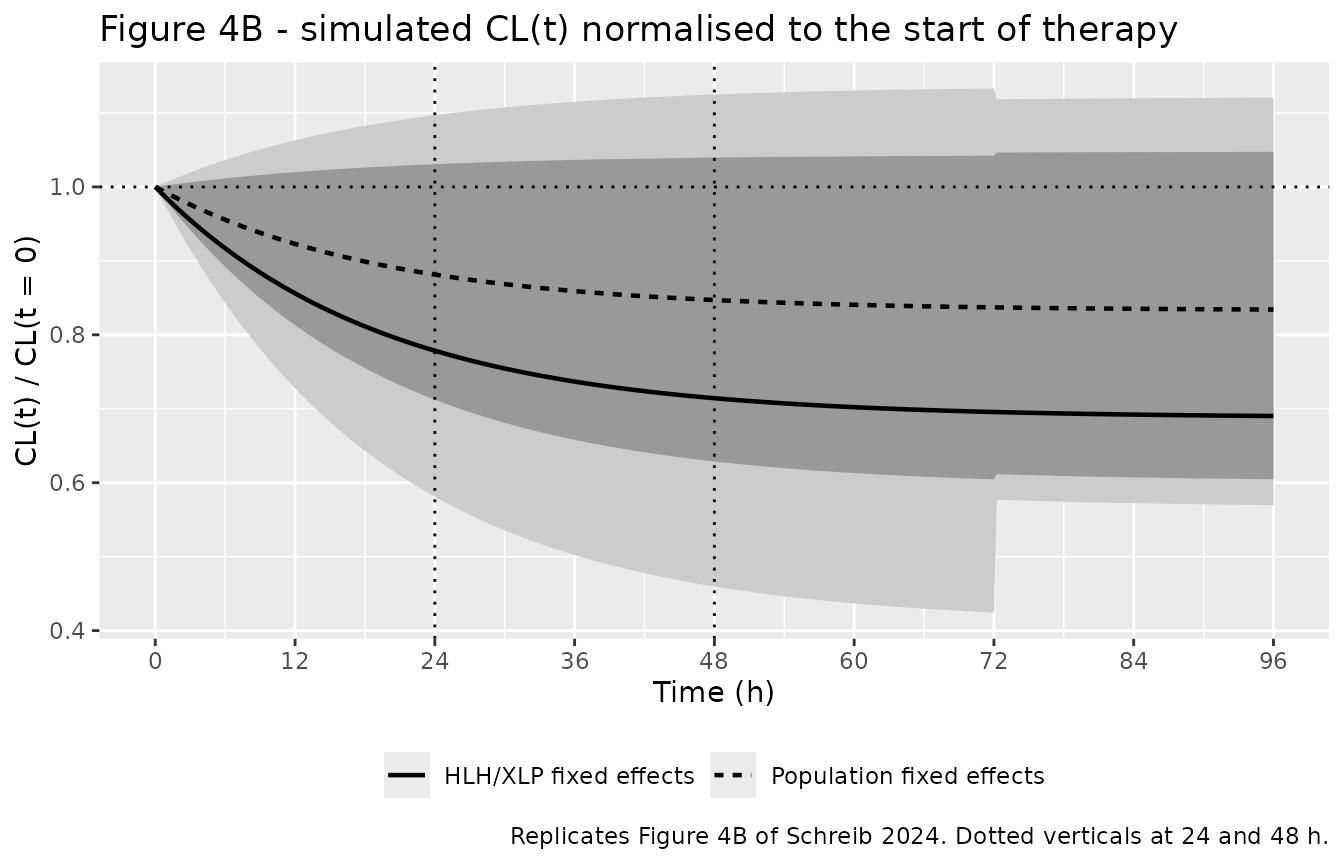
Figure 4A – distribution of weight-normalised CL at the start of therapy
Figure 4A shows the distribution of CL normalised to
body weight, in mL/min/kg, at the start of therapy.
# Replicates Figure 4A of Schreib 2024.
cl_start <- sim |>
  dplyr::filter(time == 0) |>
  dplyr::mutate(cl_ml_min_kg = kel_exp_total * vc * 1000 / 60 / WT)

ggplot(cl_start, aes(cl_ml_min_kg)) +
  geom_histogram(bins = 30, colour = "white") +
  labs(x = "CL at t = 0 (mL/min/kg)", y = "Number of subjects",
       title = "Figure 4A - weight-normalised busulfan clearance at the start of therapy",
       caption = "Replicates Figure 4A of Schreib 2024.")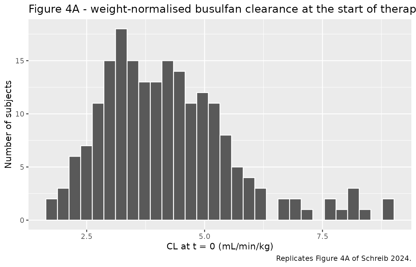
tibble::tibble(
  Statistic = c("Median", "5th percentile", "95th percentile"),
  `CL (mL/min/kg)` = round(stats::quantile(cl_start$cl_ml_min_kg,
                                           c(0.5, 0.05, 0.95)), 2)
) |>
knitr::kable(caption = "Weight-normalised clearance at the start of therapy.")| Statistic | CL (mL/min/kg) |
|---|---|
| Median | 4.02 |
| 5th percentile | 2.37 |
| 95th percentile | 6.91 |
Concentration-time profiles
sim |>
  dplyr::group_by(conditioning, time) |>
  dplyr::summarise(
    Q05 = stats::quantile(Cc, 0.05), Q50 = stats::quantile(Cc, 0.50),
    Q95 = stats::quantile(Cc, 0.95), .groups = "drop"
  ) |>
  ggplot(aes(time, Q50)) +
  geom_ribbon(aes(ymin = Q05, ymax = Q95), alpha = 0.25) +
  geom_line() +
  facet_wrap(~conditioning, ncol = 1, scales = "free_x") +
  scale_x_continuous(breaks = seq(0, 96, 12)) +
  labs(x = "Time (h)", y = "Busulfan plasma concentration (mg/L)",
       title = "Simulated twice-daily busulfan profiles by conditioning intensity",
       caption = "Median with 5th-95th percentile band.")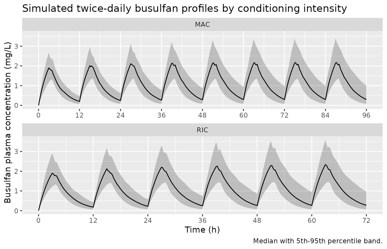
PKNCA validation
Exposure is the clinically load-bearing quantity in this paper, so the NCA is run per dosing interval. The paper gives three quantitative exposure targets to check against: a single-interval AUC of 9-12 mgh/L for the initial dose, a cumulative AUC of 45-70 mgh/L for reduced-intensity conditioning, and 80-100 mg*h/L for myeloablative conditioning (Section 2.2).
sim_nca <- sim |>
  dplyr::filter(!is.na(Cc)) |>
  dplyr::select(id, time, Cc, conditioning)

# Guarantee a time = 0 row per subject. Busulfan is given intravenously with no
# pre-existing drug, so the pre-dose concentration is 0.
sim_nca <- dplyr::bind_rows(
  sim_nca,
  sim_nca |> dplyr::distinct(id, conditioning) |>
    dplyr::mutate(time = 0, Cc = 0)
) |>
  dplyr::distinct(id, conditioning, time, .keep_all = TRUE) |>
  dplyr::arrange(id, conditioning, time)

conc_obj <- PKNCA::PKNCAconc(sim_nca, Cc ~ time | conditioning + id,
                             concu = "mg/L", timeu = "h")

dose_df <- events |>
  dplyr::filter(evid == 1) |>
  dplyr::select(id, time, amt, conditioning)
dose_obj <- PKNCA::PKNCAdose(dose_df, amt ~ time | conditioning + id,
                             doseu = "mg")

# One interval per q12h dosing interval, out to the longest regimen (8 doses).
intervals <- data.frame(
  start   = seq(0, 84, by = 12),
  end     = seq(12, 96, by = 12),
  cmax    = TRUE,
  tmax    = TRUE,
  auclast = TRUE
)

nca_res <- PKNCA::pk.nca(
  PKNCA::PKNCAdata(conc_obj, dose_obj, intervals = intervals)
)
#> Warning in .f(data_conc = .l[[1L]][[i]], data_dose = .l[[2L]][[i]],
#> data_intervals = .l[[3L]][[i]], : Error with interval start=84, end=96: No data
#> for interval
#> Warning in .f(data_conc = .l[[1L]][[i]], data_dose = .l[[2L]][[i]],
#> data_intervals = .l[[3L]][[i]], : Error with interval start=84, end=96: No data
#> for interval
#> Warning in .f(data_conc = .l[[1L]][[i]], data_dose = .l[[2L]][[i]],
#> data_intervals = .l[[3L]][[i]], : Error with interval start=84, end=96: No data
#> for interval
#> Warning in .f(data_conc = .l[[1L]][[i]], data_dose = .l[[2L]][[i]],
#> data_intervals = .l[[3L]][[i]], : Error with interval start=84, end=96: No data
#> for interval
#> Warning in .f(data_conc = .l[[1L]][[i]], data_dose = .l[[2L]][[i]],
#> data_intervals = .l[[3L]][[i]], : Error with interval start=84, end=96: No data
#> for interval
#> Warning in .f(data_conc = .l[[1L]][[i]], data_dose = .l[[2L]][[i]],
#> data_intervals = .l[[3L]][[i]], : Error with interval start=84, end=96: No data
#> for interval
#> Warning in .f(data_conc = .l[[1L]][[i]], data_dose = .l[[2L]][[i]],
#> data_intervals = .l[[3L]][[i]], : Error with interval start=84, end=96: No data
#> for interval
#> Warning in .f(data_conc = .l[[1L]][[i]], data_dose = .l[[2L]][[i]],
#> data_intervals = .l[[3L]][[i]], : Error with interval start=84, end=96: No data
#> for interval
#> Warning in .f(data_conc = .l[[1L]][[i]], data_dose = .l[[2L]][[i]],
#> data_intervals = .l[[3L]][[i]], : Error with interval start=84, end=96: No data
#> for interval
#> Warning in .f(data_conc = .l[[1L]][[i]], data_dose = .l[[2L]][[i]],
#> data_intervals = .l[[3L]][[i]], : Error with interval start=84, end=96: No data
#> for interval
#> Warning in .f(data_conc = .l[[1L]][[i]], data_dose = .l[[2L]][[i]],
#> data_intervals = .l[[3L]][[i]], : Error with interval start=84, end=96: No data
#> for interval
#> Warning in .f(data_conc = .l[[1L]][[i]], data_dose = .l[[2L]][[i]],
#> data_intervals = .l[[3L]][[i]], : Error with interval start=84, end=96: No data
#> for interval
#> Warning in .f(data_conc = .l[[1L]][[i]], data_dose = .l[[2L]][[i]],
#> data_intervals = .l[[3L]][[i]], : Error with interval start=84, end=96: No data
#> for interval
#> Warning in .f(data_conc = .l[[1L]][[i]], data_dose = .l[[2L]][[i]],
#> data_intervals = .l[[3L]][[i]], : Error with interval start=84, end=96: No data
#> for interval
#> Warning in .f(data_conc = .l[[1L]][[i]], data_dose = .l[[2L]][[i]],
#> data_intervals = .l[[3L]][[i]], : Error with interval start=84, end=96: No data
#> for interval
#> Warning in .f(data_conc = .l[[1L]][[i]], data_dose = .l[[2L]][[i]],
#> data_intervals = .l[[3L]][[i]], : Error with interval start=84, end=96: No data
#> for interval
#> Warning in .f(data_conc = .l[[1L]][[i]], data_dose = .l[[2L]][[i]],
#> data_intervals = .l[[3L]][[i]], : Error with interval start=84, end=96: No data
#> for interval
#> Warning in .f(data_conc = .l[[1L]][[i]], data_dose = .l[[2L]][[i]],
#> data_intervals = .l[[3L]][[i]], : Error with interval start=84, end=96: No data
#> for interval
#> Warning in .f(data_conc = .l[[1L]][[i]], data_dose = .l[[2L]][[i]],
#> data_intervals = .l[[3L]][[i]], : Error with interval start=84, end=96: No data
#> for interval
#> Warning in .f(data_conc = .l[[1L]][[i]], data_dose = .l[[2L]][[i]],
#> data_intervals = .l[[3L]][[i]], : Error with interval start=84, end=96: No data
#> for interval
#> Warning in .f(data_conc = .l[[1L]][[i]], data_dose = .l[[2L]][[i]],
#> data_intervals = .l[[3L]][[i]], : Error with interval start=84, end=96: No data
#> for interval
#> Warning in .f(data_conc = .l[[1L]][[i]], data_dose = .l[[2L]][[i]],
#> data_intervals = .l[[3L]][[i]], : Error with interval start=84, end=96: No data
#> for interval
#> Warning in .f(data_conc = .l[[1L]][[i]], data_dose = .l[[2L]][[i]],
#> data_intervals = .l[[3L]][[i]], : Error with interval start=84, end=96: No data
#> for interval
#> Warning in .f(data_conc = .l[[1L]][[i]], data_dose = .l[[2L]][[i]],
#> data_intervals = .l[[3L]][[i]], : Error with interval start=84, end=96: No data
#> for interval
#> Warning in .f(data_conc = .l[[1L]][[i]], data_dose = .l[[2L]][[i]],
#> data_intervals = .l[[3L]][[i]], : Error with interval start=84, end=96: No data
#> for interval
#> Warning in .f(data_conc = .l[[1L]][[i]], data_dose = .l[[2L]][[i]],
#> data_intervals = .l[[3L]][[i]], : Error with interval start=84, end=96: No data
#> for interval
#> Warning in .f(data_conc = .l[[1L]][[i]], data_dose = .l[[2L]][[i]],
#> data_intervals = .l[[3L]][[i]], : Error with interval start=84, end=96: No data
#> for interval
#> Warning in .f(data_conc = .l[[1L]][[i]], data_dose = .l[[2L]][[i]],
#> data_intervals = .l[[3L]][[i]], : Error with interval start=84, end=96: No data
#> for interval
#> Warning in .f(data_conc = .l[[1L]][[i]], data_dose = .l[[2L]][[i]],
#> data_intervals = .l[[3L]][[i]], : Error with interval start=84, end=96: No data
#> for interval
#> Warning in .f(data_conc = .l[[1L]][[i]], data_dose = .l[[2L]][[i]],
#> data_intervals = .l[[3L]][[i]], : Error with interval start=84, end=96: No data
#> for interval
#> Warning in .f(data_conc = .l[[1L]][[i]], data_dose = .l[[2L]][[i]],
#> data_intervals = .l[[3L]][[i]], : Error with interval start=84, end=96: No data
#> for interval
#> Warning in .f(data_conc = .l[[1L]][[i]], data_dose = .l[[2L]][[i]],
#> data_intervals = .l[[3L]][[i]], : Error with interval start=84, end=96: No data
#> for interval
#> Warning in .f(data_conc = .l[[1L]][[i]], data_dose = .l[[2L]][[i]],
#> data_intervals = .l[[3L]][[i]], : Error with interval start=84, end=96: No data
#> for interval
#> Warning in .f(data_conc = .l[[1L]][[i]], data_dose = .l[[2L]][[i]],
#> data_intervals = .l[[3L]][[i]], : Error with interval start=84, end=96: No data
#> for interval
#> Warning in .f(data_conc = .l[[1L]][[i]], data_dose = .l[[2L]][[i]],
#> data_intervals = .l[[3L]][[i]], : Error with interval start=84, end=96: No data
#> for interval
#> Warning in .f(data_conc = .l[[1L]][[i]], data_dose = .l[[2L]][[i]],
#> data_intervals = .l[[3L]][[i]], : Error with interval start=84, end=96: No data
#> for interval
#> Warning in .f(data_conc = .l[[1L]][[i]], data_dose = .l[[2L]][[i]],
#> data_intervals = .l[[3L]][[i]], : Error with interval start=84, end=96: No data
#> for interval
#> Warning in .f(data_conc = .l[[1L]][[i]], data_dose = .l[[2L]][[i]],
#> data_intervals = .l[[3L]][[i]], : Error with interval start=84, end=96: No data
#> for interval
#> Warning in .f(data_conc = .l[[1L]][[i]], data_dose = .l[[2L]][[i]],
#> data_intervals = .l[[3L]][[i]], : Error with interval start=84, end=96: No data
#> for interval
#> Warning in .f(data_conc = .l[[1L]][[i]], data_dose = .l[[2L]][[i]],
#> data_intervals = .l[[3L]][[i]], : Error with interval start=84, end=96: No data
#> for interval
#> Warning in .f(data_conc = .l[[1L]][[i]], data_dose = .l[[2L]][[i]],
#> data_intervals = .l[[3L]][[i]], : Error with interval start=84, end=96: No data
#> for interval
#> Warning in .f(data_conc = .l[[1L]][[i]], data_dose = .l[[2L]][[i]],
#> data_intervals = .l[[3L]][[i]], : Error with interval start=84, end=96: No data
#> for interval
#> Warning in .f(data_conc = .l[[1L]][[i]], data_dose = .l[[2L]][[i]],
#> data_intervals = .l[[3L]][[i]], : Error with interval start=84, end=96: No data
#> for interval
#> Warning in .f(data_conc = .l[[1L]][[i]], data_dose = .l[[2L]][[i]],
#> data_intervals = .l[[3L]][[i]], : Error with interval start=84, end=96: No data
#> for interval
#> Warning in .f(data_conc = .l[[1L]][[i]], data_dose = .l[[2L]][[i]],
#> data_intervals = .l[[3L]][[i]], : Error with interval start=84, end=96: No data
#> for interval
#> Warning in .f(data_conc = .l[[1L]][[i]], data_dose = .l[[2L]][[i]],
#> data_intervals = .l[[3L]][[i]], : Error with interval start=84, end=96: No data
#> for interval
#> Warning in .f(data_conc = .l[[1L]][[i]], data_dose = .l[[2L]][[i]],
#> data_intervals = .l[[3L]][[i]], : Error with interval start=84, end=96: No data
#> for interval
#> Warning in .f(data_conc = .l[[1L]][[i]], data_dose = .l[[2L]][[i]],
#> data_intervals = .l[[3L]][[i]], : Error with interval start=84, end=96: No data
#> for interval
#> Warning in .f(data_conc = .l[[1L]][[i]], data_dose = .l[[2L]][[i]],
#> data_intervals = .l[[3L]][[i]], : Error with interval start=84, end=96: No data
#> for interval
#> Warning in .f(data_conc = .l[[1L]][[i]], data_dose = .l[[2L]][[i]],
#> data_intervals = .l[[3L]][[i]], : Error with interval start=84, end=96: No data
#> for interval
#> Warning in .f(data_conc = .l[[1L]][[i]], data_dose = .l[[2L]][[i]],
#> data_intervals = .l[[3L]][[i]], : Error with interval start=84, end=96: No data
#> for interval
#> Warning in .f(data_conc = .l[[1L]][[i]], data_dose = .l[[2L]][[i]],
#> data_intervals = .l[[3L]][[i]], : Error with interval start=84, end=96: No data
#> for interval
#> Warning in .f(data_conc = .l[[1L]][[i]], data_dose = .l[[2L]][[i]],
#> data_intervals = .l[[3L]][[i]], : Error with interval start=84, end=96: No data
#> for interval
#> Warning in .f(data_conc = .l[[1L]][[i]], data_dose = .l[[2L]][[i]],
#> data_intervals = .l[[3L]][[i]], : Error with interval start=84, end=96: No data
#> for interval
#> Warning in .f(data_conc = .l[[1L]][[i]], data_dose = .l[[2L]][[i]],
#> data_intervals = .l[[3L]][[i]], : Error with interval start=84, end=96: No data
#> for interval
#> Warning in .f(data_conc = .l[[1L]][[i]], data_dose = .l[[2L]][[i]],
#> data_intervals = .l[[3L]][[i]], : Error with interval start=84, end=96: No data
#> for interval
#> Warning in .f(data_conc = .l[[1L]][[i]], data_dose = .l[[2L]][[i]],
#> data_intervals = .l[[3L]][[i]], : Error with interval start=84, end=96: No data
#> for interval
#> Warning in .f(data_conc = .l[[1L]][[i]], data_dose = .l[[2L]][[i]],
#> data_intervals = .l[[3L]][[i]], : Error with interval start=84, end=96: No data
#> for interval
#> Warning in .f(data_conc = .l[[1L]][[i]], data_dose = .l[[2L]][[i]],
#> data_intervals = .l[[3L]][[i]], : Error with interval start=84, end=96: No data
#> for interval
#> Warning in .f(data_conc = .l[[1L]][[i]], data_dose = .l[[2L]][[i]],
#> data_intervals = .l[[3L]][[i]], : Error with interval start=84, end=96: No data
#> for interval
#> Warning in .f(data_conc = .l[[1L]][[i]], data_dose = .l[[2L]][[i]],
#> data_intervals = .l[[3L]][[i]], : Error with interval start=84, end=96: No data
#> for interval
#> Warning in .f(data_conc = .l[[1L]][[i]], data_dose = .l[[2L]][[i]],
#> data_intervals = .l[[3L]][[i]], : Error with interval start=84, end=96: No data
#> for interval
#> Warning in .f(data_conc = .l[[1L]][[i]], data_dose = .l[[2L]][[i]],
#> data_intervals = .l[[3L]][[i]], : Error with interval start=84, end=96: No data
#> for interval
#> Warning in .f(data_conc = .l[[1L]][[i]], data_dose = .l[[2L]][[i]],
#> data_intervals = .l[[3L]][[i]], : Error with interval start=84, end=96: No data
#> for interval
#> Warning in .f(data_conc = .l[[1L]][[i]], data_dose = .l[[2L]][[i]],
#> data_intervals = .l[[3L]][[i]], : Error with interval start=84, end=96: No data
#> for interval
#> Warning in .f(data_conc = .l[[1L]][[i]], data_dose = .l[[2L]][[i]],
#> data_intervals = .l[[3L]][[i]], : Error with interval start=84, end=96: No data
#> for interval
#> Warning in .f(data_conc = .l[[1L]][[i]], data_dose = .l[[2L]][[i]],
#> data_intervals = .l[[3L]][[i]], : Error with interval start=84, end=96: No data
#> for interval
#> Warning in .f(data_conc = .l[[1L]][[i]], data_dose = .l[[2L]][[i]],
#> data_intervals = .l[[3L]][[i]], : Error with interval start=84, end=96: No data
#> for interval
#> Warning in .f(data_conc = .l[[1L]][[i]], data_dose = .l[[2L]][[i]],
#> data_intervals = .l[[3L]][[i]], : Error with interval start=84, end=96: No data
#> for interval
#> Warning in .f(data_conc = .l[[1L]][[i]], data_dose = .l[[2L]][[i]],
#> data_intervals = .l[[3L]][[i]], : Error with interval start=84, end=96: No data
#> for interval
#> Warning in .f(data_conc = .l[[1L]][[i]], data_dose = .l[[2L]][[i]],
#> data_intervals = .l[[3L]][[i]], : Error with interval start=84, end=96: No data
#> for interval
#> Warning in .f(data_conc = .l[[1L]][[i]], data_dose = .l[[2L]][[i]],
#> data_intervals = .l[[3L]][[i]], : Error with interval start=84, end=96: No data
#> for interval
#> Warning in .f(data_conc = .l[[1L]][[i]], data_dose = .l[[2L]][[i]],
#> data_intervals = .l[[3L]][[i]], : Error with interval start=84, end=96: No data
#> for interval
#> Warning in .f(data_conc = .l[[1L]][[i]], data_dose = .l[[2L]][[i]],
#> data_intervals = .l[[3L]][[i]], : Error with interval start=84, end=96: No data
#> for interval
#> Warning in .f(data_conc = .l[[1L]][[i]], data_dose = .l[[2L]][[i]],
#> data_intervals = .l[[3L]][[i]], : Error with interval start=84, end=96: No data
#> for interval
#> Warning in .f(data_conc = .l[[1L]][[i]], data_dose = .l[[2L]][[i]],
#> data_intervals = .l[[3L]][[i]], : Error with interval start=84, end=96: No data
#> for interval
#> Warning in .f(data_conc = .l[[1L]][[i]], data_dose = .l[[2L]][[i]],
#> data_intervals = .l[[3L]][[i]], : Error with interval start=84, end=96: No data
#> for interval
#> Warning in .f(data_conc = .l[[1L]][[i]], data_dose = .l[[2L]][[i]],
#> data_intervals = .l[[3L]][[i]], : Error with interval start=84, end=96: No data
#> for interval
#> Warning in .f(data_conc = .l[[1L]][[i]], data_dose = .l[[2L]][[i]],
#> data_intervals = .l[[3L]][[i]], : Error with interval start=84, end=96: No data
#> for interval
#> Warning in .f(data_conc = .l[[1L]][[i]], data_dose = .l[[2L]][[i]],
#> data_intervals = .l[[3L]][[i]], : Error with interval start=84, end=96: No data
#> for interval
#> Warning in .f(data_conc = .l[[1L]][[i]], data_dose = .l[[2L]][[i]],
#> data_intervals = .l[[3L]][[i]], : Error with interval start=84, end=96: No data
#> for interval
#> Warning in .f(data_conc = .l[[1L]][[i]], data_dose = .l[[2L]][[i]],
#> data_intervals = .l[[3L]][[i]], : Error with interval start=84, end=96: No data
#> for interval
#> Warning in .f(data_conc = .l[[1L]][[i]], data_dose = .l[[2L]][[i]],
#> data_intervals = .l[[3L]][[i]], : Error with interval start=84, end=96: No data
#> for interval
#> Warning in .f(data_conc = .l[[1L]][[i]], data_dose = .l[[2L]][[i]],
#> data_intervals = .l[[3L]][[i]], : Error with interval start=84, end=96: No data
#> for interval
#> Warning in .f(data_conc = .l[[1L]][[i]], data_dose = .l[[2L]][[i]],
#> data_intervals = .l[[3L]][[i]], : Error with interval start=84, end=96: No data
#> for interval
#> Warning in .f(data_conc = .l[[1L]][[i]], data_dose = .l[[2L]][[i]],
#> data_intervals = .l[[3L]][[i]], : Error with interval start=84, end=96: No data
#> for interval
#> Warning in .f(data_conc = .l[[1L]][[i]], data_dose = .l[[2L]][[i]],
#> data_intervals = .l[[3L]][[i]], : Error with interval start=84, end=96: No data
#> for interval
#> Warning in .f(data_conc = .l[[1L]][[i]], data_dose = .l[[2L]][[i]],
#> data_intervals = .l[[3L]][[i]], : Error with interval start=84, end=96: No data
#> for interval
#> Warning in .f(data_conc = .l[[1L]][[i]], data_dose = .l[[2L]][[i]],
#> data_intervals = .l[[3L]][[i]], : Error with interval start=84, end=96: No data
#> for interval
#> Warning in .f(data_conc = .l[[1L]][[i]], data_dose = .l[[2L]][[i]],
#> data_intervals = .l[[3L]][[i]], : Error with interval start=84, end=96: No data
#> for interval
#> Warning in .f(data_conc = .l[[1L]][[i]], data_dose = .l[[2L]][[i]],
#> data_intervals = .l[[3L]][[i]], : Error with interval start=84, end=96: No data
#> for interval
#> Warning in .f(data_conc = .l[[1L]][[i]], data_dose = .l[[2L]][[i]],
#> data_intervals = .l[[3L]][[i]], : Error with interval start=84, end=96: No data
#> for interval
#> Warning in .f(data_conc = .l[[1L]][[i]], data_dose = .l[[2L]][[i]],
#> data_intervals = .l[[3L]][[i]], : Error with interval start=84, end=96: No data
#> for interval
#> Warning in .f(data_conc = .l[[1L]][[i]], data_dose = .l[[2L]][[i]],
#> data_intervals = .l[[3L]][[i]], : Error with interval start=84, end=96: No data
#> for interval
#> Warning in .f(data_conc = .l[[1L]][[i]], data_dose = .l[[2L]][[i]],
#> data_intervals = .l[[3L]][[i]], : Error with interval start=84, end=96: No data
#> for interval
#> Warning in .f(data_conc = .l[[1L]][[i]], data_dose = .l[[2L]][[i]],
#> data_intervals = .l[[3L]][[i]], : Error with interval start=84, end=96: No data
#> for interval
#> Warning in .f(data_conc = .l[[1L]][[i]], data_dose = .l[[2L]][[i]],
#> data_intervals = .l[[3L]][[i]], : Error with interval start=84, end=96: No data
#> for interval
#> Warning in .f(data_conc = .l[[1L]][[i]], data_dose = .l[[2L]][[i]],
#> data_intervals = .l[[3L]][[i]], : Error with interval start=84, end=96: No data
#> for interval
#> Warning in .f(data_conc = .l[[1L]][[i]], data_dose = .l[[2L]][[i]],
#> data_intervals = .l[[3L]][[i]], : Error with interval start=84, end=96: No data
#> for interval
#> Warning in .f(data_conc = .l[[1L]][[i]], data_dose = .l[[2L]][[i]],
#> data_intervals = .l[[3L]][[i]], : Error with interval start=84, end=96: No data
#> for interval
#> Warning in .f(data_conc = .l[[1L]][[i]], data_dose = .l[[2L]][[i]],
#> data_intervals = .l[[3L]][[i]], : Error with interval start=84, end=96: No data
#> for interval
#> Warning in .f(data_conc = .l[[1L]][[i]], data_dose = .l[[2L]][[i]],
#> data_intervals = .l[[3L]][[i]], : Error with interval start=84, end=96: No data
#> for interval
#> Warning in .f(data_conc = .l[[1L]][[i]], data_dose = .l[[2L]][[i]],
#> data_intervals = .l[[3L]][[i]], : Error with interval start=84, end=96: No data
#> for interval
#> Warning in .f(data_conc = .l[[1L]][[i]], data_dose = .l[[2L]][[i]],
#> data_intervals = .l[[3L]][[i]], : Error with interval start=84, end=96: No data
#> for interval
#> Warning in .f(data_conc = .l[[1L]][[i]], data_dose = .l[[2L]][[i]],
#> data_intervals = .l[[3L]][[i]], : Error with interval start=84, end=96: No data
#> for interval
#> Warning in .f(data_conc = .l[[1L]][[i]], data_dose = .l[[2L]][[i]],
#> data_intervals = .l[[3L]][[i]], : Error with interval start=84, end=96: No data
#> for interval
#> Warning in .f(data_conc = .l[[1L]][[i]], data_dose = .l[[2L]][[i]],
#> data_intervals = .l[[3L]][[i]], : Error with interval start=84, end=96: No data
#> for interval
#> Warning in .f(data_conc = .l[[1L]][[i]], data_dose = .l[[2L]][[i]],
#> data_intervals = .l[[3L]][[i]], : Error with interval start=84, end=96: No data
#> for interval
#> Warning in .f(data_conc = .l[[1L]][[i]], data_dose = .l[[2L]][[i]],
#> data_intervals = .l[[3L]][[i]], : Error with interval start=84, end=96: No data
#> for interval
#> Warning in .f(data_conc = .l[[1L]][[i]], data_dose = .l[[2L]][[i]],
#> data_intervals = .l[[3L]][[i]], : Error with interval start=84, end=96: No data
#> for interval
#> Warning in .f(data_conc = .l[[1L]][[i]], data_dose = .l[[2L]][[i]],
#> data_intervals = .l[[3L]][[i]], : Error with interval start=84, end=96: No data
#> for interval
#> Warning in .f(data_conc = .l[[1L]][[i]], data_dose = .l[[2L]][[i]],
#> data_intervals = .l[[3L]][[i]], : Error with interval start=84, end=96: No data
#> for interval
#> Warning in .f(data_conc = .l[[1L]][[i]], data_dose = .l[[2L]][[i]],
#> data_intervals = .l[[3L]][[i]], : Error with interval start=84, end=96: No data
#> for interval
#> Warning in .f(data_conc = .l[[1L]][[i]], data_dose = .l[[2L]][[i]],
#> data_intervals = .l[[3L]][[i]], : Error with interval start=84, end=96: No data
#> for interval
#> Warning in .f(data_conc = .l[[1L]][[i]], data_dose = .l[[2L]][[i]],
#> data_intervals = .l[[3L]][[i]], : Error with interval start=84, end=96: No data
#> for interval
#> Warning in .f(data_conc = .l[[1L]][[i]], data_dose = .l[[2L]][[i]],
#> data_intervals = .l[[3L]][[i]], : Error with interval start=84, end=96: No data
#> for interval
#> Warning in .f(data_conc = .l[[1L]][[i]], data_dose = .l[[2L]][[i]],
#> data_intervals = .l[[3L]][[i]], : Error with interval start=84, end=96: No data
#> for interval
#> Warning in .f(data_conc = .l[[1L]][[i]], data_dose = .l[[2L]][[i]],
#> data_intervals = .l[[3L]][[i]], : Error with interval start=84, end=96: No data
#> for interval
#> Warning in .f(data_conc = .l[[1L]][[i]], data_dose = .l[[2L]][[i]],
#> data_intervals = .l[[3L]][[i]], : Error with interval start=84, end=96: No data
#> for interval
#> Warning in .f(data_conc = .l[[1L]][[i]], data_dose = .l[[2L]][[i]],
#> data_intervals = .l[[3L]][[i]], : Error with interval start=84, end=96: No data
#> for interval

nca_df <- as.data.frame(nca_res) |>
  dplyr::filter(!is.na(PPORRES))
Per-interval AUC and the accumulation the model predicts
Because the elimination rate constant falls over the course of
therapy while the dose is held fixed, exposure per dosing interval must
rise. The model makes an exact quantitative prediction for that
rise: at the asymptote,
AUC(late) / AUC(first) = 1 / (1 + dk), which is
1 / 0.833 = 1.20 for the population and
1 / 0.688 = 1.45 for the HLH/XLP group. This is the
pharmacological content of the paper’s conclusion that repeated PK
assessment is essential, and it is a falsifiable prediction rather than
a restatement of the dosing input: only the first interval was
dosed to target, so every later interval’s exposure is an out-of-sample
prediction of the model.
interval_auc <- nca_df |>
  dplyr::filter(PPTESTCD == "auclast") |>
  dplyr::mutate(dose_no = as.integer(start / 12) + 1L) |>
  dplyr::left_join(
    subjects |> dplyr::select(id, DIS_HLHXLP), by = "id"
  )

interval_auc |>
  dplyr::group_by(conditioning, dose_no) |>
  dplyr::summarise(`Median AUC (mg*h/L)` = round(stats::median(PPORRES), 2),
                   .groups = "drop") |>
  tidyr::pivot_wider(names_from = conditioning,
                     values_from = `Median AUC (mg*h/L)`) |>
  dplyr::rename(`Dosing interval` = dose_no) |>
  knitr::kable(
    caption = paste(
      "Median AUC per q12h dosing interval. The first interval is dosed to the",
      "paper's 9-12 mg*h/L target (midpoint 10.5); later intervals rise because",
      "clearance falls. RIC regimens stop after 6 doses."
    )
)| Dosing interval | MAC | RIC |
|---|---|---|
| 1 | 10.72 | 10.54 |
| 2 | 12.46 | 12.07 |
| 3 | 12.93 | 12.66 |
| 4 | 13.19 | 12.98 |
| 5 | 13.34 | 13.37 |
| 6 | 13.49 | 13.57 |
| 7 | 13.50 | NA |
| 8 | 13.51 | NA |
# Typical-value (random effects zeroed) accumulation for the two diagnosis
# groups, over the same 6-dose reduced-intensity regimen, so the comparison
# against the asymptote is like-for-like. HLH/XLP patients are all in the RIC
# arm of this cohort.
typ_ratio <- function(hlhxlp) {
  ev <- trap_ev |> dplyr::mutate(DIS_HLHXLP = hlhxlp)
  a <- interval_auc_of(
    rxode2::rxSolve(rxode2::zeroRe(mod), ev, returnType = "data.frame",
                    omega = NA, useLinCmt = FALSE))
  a[6] / a[1]
}

interval_auc |>
  dplyr::filter(conditioning == "RIC") |>
  dplyr::mutate(group = ifelse(DIS_HLHXLP == 1, "HLH/XLP", "All others")) |>
  dplyr::group_by(id, group) |>
  dplyr::summarise(ratio = PPORRES[which.max(dose_no)] / PPORRES[which.min(dose_no)],
                   .groups = "drop") |>
  dplyr::group_by(group) |>
  dplyr::summarise(
    n = dplyr::n(),
    `Population median` = round(stats::median(ratio), 3),
    .groups = "drop"
  ) |>
  dplyr::mutate(
    `Typical value` = round(c(typ_ratio(0), typ_ratio(1))[match(group, c("All others", "HLH/XLP"))], 3),
    `Asymptote 1/(1+dk)` = ifelse(group == "HLH/XLP",
                                  round(1 / (1 - 0.312), 3),
                                  round(1 / (1 - 0.167), 3))
  ) |>
  dplyr::rename(Group = group, N = n) |>
  dplyr::relocate(`Typical value`, .before = `Population median`) |>
  knitr::kable(
    caption = paste(
      "Accumulation of per-interval exposure over the 6-dose reduced-intensity",
      "regimen: AUC of the last interval divided by AUC of the first. The",
      "typical-value column approaches but does not reach the asymptote,",
      "because kappa_k gives the change a 13.4 h half-life while the regimen",
      "runs only three days. The population median sits ABOVE the typical value",
      "because the random effect on kel_exp_famp enters exposure as",
      "1/(1 + dk) -- a strongly right-skewed transformation, so the median of",
      "the resulting exposure ratio is pulled up relative to the ratio at the",
      "median dk."
    )
)| Group | N | Typical value | Population median | Asymptote 1/(1+dk) |
|---|---|---|---|---|
| All others | 97 | 1.188 | 1.251 | 1.200 |
| HLH/XLP | 23 | 1.389 | 1.492 | 1.453 |
Cumulative AUC against the published conditioning targets
The cohort below is dosed once, to the paper’s 9-12 mg*h/L first-interval target, and never re-assessed. That is deliberately the scenario Schreib 2024 argues against, so the expected result is a cumulative overshoot of the conditioning-intensity target rather than a match to it: exposure per interval climbs about 20-25% as clearance falls, and nothing corrects for it. Reading the table below as a validation failure would be a misreading – the overshoot is the quantitative content of the paper’s conclusion that “repeated pharmacokinetic assessment [is] essential to achieve the desired target exposure in twice-daily busulfan administration.”
cauc <- interval_auc |>
  dplyr::group_by(id, conditioning) |>
  dplyr::summarise(cAUC = sum(PPORRES), .groups = "drop")

published_targets <- tibble::tibble(
  conditioning = c("MAC", "RIC"),
  `Target cAUC (mg*h/L)` = c("80-100", "45-70"),
  `Doses simulated` = c(8L, 6L)
)

cauc |>
  dplyr::group_by(conditioning) |>
  dplyr::summarise(
    N = dplyr::n(),
    `Median cAUC (mg*h/L)` = round(stats::median(cAUC), 1),
    `5th-95th percentile` = sprintf("%.1f-%.1f",
                                    stats::quantile(cAUC, 0.05),
                                    stats::quantile(cAUC, 0.95)),
    .groups = "drop"
  ) |>
  dplyr::left_join(published_targets, by = "conditioning") |>
  dplyr::rename(Conditioning = conditioning) |>
  knitr::kable(
    caption = paste(
      "Simulated cumulative AUC versus the conditioning-intensity targets in",
      "Section 2.2 of Schreib 2024. Doses were set from the first-interval",
      "target only, with no subsequent therapeutic drug monitoring."
    )
)| Conditioning | N | Median cAUC (mg*h/L) | 5th-95th percentile | Target cAUC (mg*h/L) | Doses simulated |
|---|---|---|---|---|---|
| MAC | 80 | 103.6 | 61.6-161.0 | 80-100 | 8 |
| RIC | 120 | 75.5 | 47.3-122.8 | 45-70 | 6 |
Single-interval NCA against the published initial-dose target
first_interval <- nca_df |>
  dplyr::filter(start == 0) |>
  dplyr::group_by(conditioning, PPTESTCD) |>
  dplyr::summarise(PPORRES = stats::median(PPORRES), .groups = "drop") |>
  tidyr::pivot_wider(names_from = PPTESTCD, values_from = PPORRES)

# Schreib 2024 Section 2.2: the initial dose targeted an AUC of 9-12 mg*h/L.
# The midpoint, 10.5, is the reference the doses were set to.
published <- tibble::tibble(
  conditioning = c("MAC", "RIC"),
  auclast      = c(10.5, 10.5)
)

cmp <- nlmixr2lib::ncaComparisonTable(
  simulated     = first_interval,
  reference     = published,
  by            = "conditioning",
  params        = "auclast",
  units         = c(auclast = "mg*h/L"),
  tolerance_pct = 20
)

knitr::kable(
  cmp,
  caption = paste(
    "First-interval AUC versus the 9-12 mg*h/L initial-dose target of Schreib",
    "2024 Section 2.2. * marks a >20% difference from the reference."
  )
)| NCA parameter | conditioning | Reference | Simulated | % diff |
|---|---|---|---|---|
| AUClast (mg*h/L) | MAC | 10.5 | 10.7 | +2.1% |
| AUClast (mg*h/L) | RIC | 10.5 | 10.5 | +0.3% |
The paper reports no tabulated NCA summary in the main text; the
non-parametric AUC, Cmax, CL,
V, t1/2 and MRT values computed
in Section 2.6 appear only in Table S1 and Figures S4-S9 of the
supplement, which was not available when this model was built. The
comparison above therefore uses the explicitly stated exposure targets
of Section 2.2 rather than a transcribed NCA table.
Assumptions and deviations
-
useLinCmt = FALSEon rxode2 5.1.6 and earlier. The model is one-compartment with linear elimination, sorxSolve()’s default ODE-to-linCmt()conversion used to replace it with a closed form that can only hold a constant elimination rate constant, silently discarding the time dependence and under-predicting steady-state exposure per interval by about 17% (45% in the HLH/XLP group). Rewriting the ODE did not help: an explicit rate variable and a clearance-form denominator were both tested and were converted identically, so the flag was the only mitigation. rxode2 now 5.1.7 refuses the conversion when it would change the model and the flag is no longer required; this vignette keeps it so that it stays correct on older installations. This was always a property of the solver’s default, not of the published model. -
Equation (2), not Equation (3). The packaged model
integrates the instantaneous rate constant
k*(t)of Equation (2). Equation (3)‘sk'(t)is a running time-average that exists only to givesaemixa closed-form likelihood without an ODE solver. The choice is falsified against Figure 4B above and against the authors’ ownkchange.R, which calls stepwise integration ofk*(t)“the reference”. -
Continuous time, not the dosing-interval midpoint.
Equation (2) as printed evaluates the exponential at
t_mid, the midpoint of the dosing interval, and the deposited fit functionBuFunD.Rimplements that asTimeAv <- (ceiling(Time/12) - 0.5) * 12. The packaged model uses continuoustimeinstead, for two reasons: the published Figure 4B starts at exactly 1.0 att = 0and is smooth, whereas the discretised form would start at 0.956; and a hard-coded 12 h interval would silently corrupt any simulation that is not q12h. The AUC difference between the two forms is about 1%. -
Transposed exponents in Table 3. The multiplicative
rewrite of the
ln(k)equation printed in Table 3 readsk = e^theta_k1 * Fmat^theta_k2 * (TBW/(10 L))^theta_k3 * ..., transposingtheta_k2andtheta_k3relative to the additive form printed directly above it. The additive form is correct and is what the model encodes. Three independent checks agree: Table 3’s own row labels (“theta_k2, effect of dln(TBW, L)” with reference value 10 L; “theta_k3, effect of ln(Fmat)” with reference value 0), Table 2’s model-building sequence (model 15 adds ln(TBW) on ln(k) astheta_k2; model 16** adds ln(Fmat) astheta_k3), and the tabulated population range of thetheta_k3term (-0.40 to 0), which is only possible for a non-negative coefficient onln(Fmat)becauseFmat <= 1. -
Units of
dkin Table 3. Thetheta_dk1row is labelled “dk(h-1)”, butdkis a dimensionless fraction: the surrounding text describes it as “an average reduction in k and CL by 16.7 +/- 18.0%”. The model treats it as dimensionless. - The ALL sentence uses the wrong base. Section 3.2 states “ALL significantly reduced k by 20% on average (100 x (1 - 10^-0.21)”. With base 10 the reduction would be 38%, not 20%; with base e it is 18.9%, which is what the sentence claims and what the model encodes.
-
Postmenstrual-age conversion. The Methods state
only that postmenstrual age is postnatal age plus a fixed 40 weeks. The
52-weeks-per-year conversion is taken from the deposited
BuSaemix.R(Fmat = 1/(1 + ((age + 40/52)/(46/52))^-2.3)). It is confirmed independently by the paper’s own statement thatFmatis 0.85 at 98 weeks postmenstrual age: the packaged model returns 0.851. -
Height is a derived covariate. Schreib 2024
recorded body surface area, not height, and back-calculated height by
inverting Equation (6). The model takes
HTin cm directly; the virtual cohort reproduces the authors’ route by generating BSA from weight and inverting Mosteller. - Virtual-cohort distributions. Age, weight, albumin, infusion duration, sex and the two disease indicators are sampled to match the Table 1 marginals; the joint distribution is not published. The median weight-for-age curve is an assumption, calibrated to pass through the cohort medians (17.2 kg at 4.3 years). The 3 h / 4 h infusion split is set to 50/50 because the per-protocol patient counts appear only in Figure S1, which was not available when this model was built. Disease indicators are assigned within conditioning arms (ALL to myeloablative, HLH/XLP to reduced intensity) at within-arm prevalences that reproduce the whole-cohort 10% and 11%.
- Dosing. Doses are set from the model itself to the midpoint of the paper’s 9-12 mgh/L first-interval target, using population parameters with the random effects zeroed, because a prescriber does not know a patient’s random effects. No subsequent therapeutic drug monitoring is simulated, so the cumulative AUCs above show what happens when the initial dose is not* adjusted – which is precisely the scenario the paper’s conclusion argues against.
-
TINFis supplied twice. Infusion duration is both a covariate onln(V)andln(k)and the physical duration of the dose record. rxode2 takes the physical duration from the event table’sdurcolumn and does not expose it tomodel(), so the event tables setdur = TINFand also carryTINFas a covariate column. -
No covariances between random effects. Table 3
reports three variances and no covariances, so the packaged OMEGA is
diagonal. Random effects on
ln(kappa_k)were dropped by the authors because their shrinkage exceeded 60% (Table 2, model 2 versus model 3*). - Residual error is additive. Schreib 2024 tested a proportional error model and rejected it: it failed to compute -2LL and gave an asymmetric residual distribution (Sections 2.5 and 3.3).
-
Excluded covariates. Hematocrit on
ln(V)and leukocyte count onln(k)reached forward-selection significance but failed backward elimination (Table 2, step 3) and are not in the final model. N-acetylcysteine onln(V)came close to the inclusion criteria (a roughly 10% increase in V) but its effect size fell just under the 0.1 threshold at 0.099. None of these are encoded.