Tadalafil (Ferguson-Sells 2022)
Source:vignettes/articles/FergusonSells_2022_tadalafil.Rmd
FergusonSells_2022_tadalafil.RmdModel and source
- Citation: Ferguson-Sells L, Velez de Mendizabal N, Li B, Small D. Population Pharmacokinetics of Tadalafil in Pediatric Patients with Pulmonary Arterial Hypertension: A Combined Adult/Pediatric Model. Clin Pharmacokinet. 2022;61(2):249-262. doi:10.1007/s40262-021-01052-8
- Description: One-compartment population PK model with first-order absorption for oral tadalafil in adult and pediatric patients (2 to < 18 years) with pulmonary arterial hypertension, fitted to pooled PHIRST-1 (adults) and H6D-MC-LVIG (children) data. Apparent clearance is higher in patients taking concomitant bosentan (a CYP3A inducer), apparent volume scales linearly with body weight (exponent fixed to 1, reference 70 kg), and relative bioavailability is a power function of dose (falling with increasing dose) and of age (falling with decreasing age). Clearance has no weight effect. Residual error is combined proportional plus additive.
- Article: https://doi.org/10.1007/s40262-021-01052-8 (open access, PMC8813705)
Population
The model was fitted to 1430 plasma tadalafil concentrations from 324 patients with pulmonary arterial hypertension (PAH) pooled from two studies (Ferguson-Sells 2022 Table 1 and Results):
- PHIRST-1 (NCT00125918): 305 adults (69 male, 236 female; 1102 observations), median age 53.9 years (14.7-90.3), median weight 73.0 kg (41.4-140), randomised to 2.5, 10, 20 or 40 mg tablet once daily, with sparse sampling at weeks 4, 8, 12 and 16.
- LVIG (NCT01484431): 19 children aged 2.5 to 18 years (6 male, 13 female; 328 observations) in three weight cohorts – heavy (>= 40 kg, n = 6, median 49.0 kg, 14.6 years), middle (25 to < 40 kg, n = 7, median 30.1 kg, 11.0 years) and light (< 25 kg, n = 6, median 14.7 kg, 5.0 years). Each child received a low dose for 5 weeks and then a high dose for 5 weeks; the light-weight cohort received a 2 mg/mL oral suspension and the other cohorts received tablets. Serial samples were collected at predose and 2, 4, 8, 12 and 24 h on day 1, day 14 and day 49.
About half of the adults and of the children took concomitant
bosentan, a CYP3A inducer. Patients taking ambrisentan were grouped with
non-bosentan patients. The same information is available
programmatically via
readModelDb("FergusonSells_2022_tadalafil")()$population.
Source trace
Every ini() value carries an in-file source comment in
inst/modeldb/specificDrugs/FergusonSells_2022_tadalafil.R.
They are collected here.
| Equation / parameter | Value | Source location |
|---|---|---|
lka |
log(0.860) 1/h | Table 2, Ka |
lcl (CL/F, taking bosentan) |
log(3.23) L/h | Table 2, ‘Patients taking bosentan’ |
e_conmed_bosentan_cl |
-0.418 | Table 2, ‘Effect of non-bosentan’ |
lvc (V/F at 70 kg) |
log(88.1) L | Table 2, ‘V/F 70 kg patient’ |
e_wt_vc |
1 (fixed) | Table 2, ‘Effect of weight’ |
lfdepot |
log(1) (fixed) | Table 2, ‘F’ |
e_dose_fdepot |
-0.227 | Table 2, ‘Effect of dose (continuous) on F’ |
e_age_fdepot |
0.100 | Table 2, ‘Effect of age on F’ |
etalka |
log(1 + 2.01^2) = 1.617 | Table 2, Ka IIV 201% CV (footnote b) |
etalcl |
log(1 + 0.485^2) = 0.211 | Table 2, CL/F IIV 48.5% CV (footnote b) |
etalvc |
log(1 + 0.321^2) = 0.0981 | Table 2, V/F IIV 32.1% CV (footnote b) |
propSd |
0.258 | Table 2, residual error ‘Proportional’ (footnote f) |
addSd |
11.6 ng/mL | Table 2, residual error ‘Additive’ (footnote f) |
| CL/F equation | CL = TVCL * BOS + TVCL * (1 + EffNoBos) * (1 - BOS) |
Table 2 footnote c |
| V/F equation | V = TVV * (WT/70)^EffWt |
Table 2 footnote d |
| F equation | F = TVF * (DOSE/16.27)^EffDoseF * (AGEE/52.4)^EffAgeF |
Table 2 footnote e |
| Structure | one compartment, first-order absorption and elimination | Methods 2.3 |
Typical-value check against Table 3
Ferguson-Sells 2022 Table 3 reports the model-predicted CL/F, V/F,
AUC over the dosing interval and half-life for a typical adult and for a
patient at the median weight and age of each pediatric cohort, at the
proposed phase III dose. Because the model applies bioavailability
explicitly, the apparent parameters Table 3 prints are
CL / F and V / F with F evaluated
at that dose and age. Table 3 gives the median of a 10,000-patient
simulation; the medians of log-normal CL and V
equal their typical values, so a closed-form typical-value calculation
is directly comparable.
mod <- readModelDb("FergusonSells_2022_tadalafil")
th <- rxode2::rxode(mod)$theta
#> ℹ parameter labels from comments will be replaced by 'label()'

cohorts <- tibble::tribble(
  ~cohort,                  ~WT,  ~AGE, ~DOSE,
  "Typical adult",          70.0, 54,   40,
  "Heavy-weight (>= 40 kg)", 49.0, 14.6, 40,
  "Middle-weight (25-40 kg)", 30.1, 11.0, 20,
  "Light-weight (< 25 kg)",  14.7, 5.0,  20
)
cohort_levels <- cohorts$cohort

# Table 3, pediatric-model rows: CL/F (L/h), V/F (L), AUCtau (ng*h/mL),
# Cmean,ss (ng/mL), half-life (h).
table3 <- tibble::tribble(
  ~bosentan, ~cohort,                    ~cl_f, ~v_f,  ~auc,  ~cmean, ~thalf,
  "No",      "Typical adult",            2.33,  107,   17100, 714,    32.0,
  "No",      "Heavy-weight (>= 40 kg)",  2.63,  85.6,  15200, 633,    22.6,
  "No",      "Middle-weight (25-40 kg)", 2.38,  45.7,  8390,  350,    13.5,
  "No",      "Light-weight (< 25 kg)",   2.45,  24.6,  8170,  340,    6.94,
  "Yes",     "Typical adult",            4.05,  107,   9870,  411,    18.5,
  "Yes",     "Heavy-weight (>= 40 kg)",  4.45,  86.9,  8990,  375,    13.3,
  "Yes",     "Middle-weight (25-40 kg)", 4.00,  46.8,  5000,  209,    8.08,
  "Yes",     "Light-weight (< 25 kg)",   4.39,  24.5,  4550,  190,    3.78
)

typical <- tidyr::crossing(cohorts, bosentan = c("No", "Yes")) |>
  dplyr::mutate(
    CONMED_BOSENTAN = as.integer(bosentan == "Yes"),
    fdepot = exp(th[["lfdepot"]]) * (DOSE / 16.27)^th[["e_dose_fdepot"]] *
      (AGE / 52.4)^th[["e_age_fdepot"]],
    cl = exp(th[["lcl"]]) *
      (1 + th[["e_conmed_bosentan_cl"]] * (1 - CONMED_BOSENTAN)),
    vc = exp(th[["lvc"]]) * (WT / 70)^th[["e_wt_vc"]],
    cl_f_model = cl / fdepot,
    v_f_model = vc / fdepot,
    auc_model = 1000 * DOSE / cl_f_model,
    thalf_model = log(2) * vc / cl
  ) |>
  dplyr::inner_join(table3, by = c("bosentan", "cohort")) |>
  dplyr::mutate(
    cohort = factor(cohort, levels = cohort_levels),
    pct_cl = 100 * (cl_f_model / cl_f - 1),
    pct_v = 100 * (v_f_model / v_f - 1),
    pct_auc = 100 * (auc_model / auc - 1),
    pct_thalf = 100 * (thalf_model / thalf - 1)
  ) |>
  dplyr::arrange(bosentan, cohort)

typical |>
  dplyr::transmute(
    bosentan, cohort, DOSE, fdepot = signif(fdepot, 3),
    cl_f_model = signif(cl_f_model, 3), cl_f,
    v_f_model = signif(v_f_model, 3), v_f,
    auc_model = signif(auc_model, 3), auc,
    thalf_model = signif(thalf_model, 3), thalf
  ) |>
  dplyr::rename(
    "Bosentan" = bosentan, "Cohort" = cohort, "Dose (mg)" = DOSE,
    "F" = fdepot,
    "CL/F model (L/h)" = cl_f_model, "CL/F Table 3" = cl_f,
    "V/F model (L)" = v_f_model, "V/F Table 3" = v_f,
    "AUCtau model (ng*h/mL)" = auc_model, "AUCtau Table 3" = auc,
    "t1/2 model (h)" = thalf_model, "t1/2 Table 3" = thalf
  ) |>
knitr::kable(caption = "Typical-value apparent parameters vs. Table 3 medians.")| Bosentan | Cohort | Dose (mg) | F | CL/F model (L/h) | CL/F Table 3 | V/F model (L) | V/F Table 3 | AUCtau model (ng*h/mL) | AUCtau Table 3 | t1/2 model (h) | t1/2 Table 3 |
|---|---|---|---|---|---|---|---|---|---|---|---|
| No | Typical adult | 40 | 0.818 | 2.30 | 2.33 | 108.0 | 107.0 | 17400 | 17100 | 32.50 | 32.00 |
| No | Heavy-weight (>= 40 kg) | 40 | 0.717 | 2.62 | 2.63 | 86.0 | 85.6 | 15300 | 15200 | 22.70 | 22.60 |
| No | Middle-weight (25-40 kg) | 20 | 0.816 | 2.30 | 2.38 | 46.4 | 45.7 | 8680 | 8390 | 14.00 | 13.50 |
| No | Light-weight (< 25 kg) | 20 | 0.754 | 2.49 | 2.45 | 24.5 | 24.6 | 8030 | 8170 | 6.82 | 6.94 |
| Yes | Typical adult | 40 | 0.818 | 3.95 | 4.05 | 108.0 | 107.0 | 10100 | 9870 | 18.90 | 18.50 |
| Yes | Heavy-weight (>= 40 kg) | 40 | 0.717 | 4.50 | 4.45 | 86.0 | 86.9 | 8890 | 8990 | 13.20 | 13.30 |
| Yes | Middle-weight (25-40 kg) | 20 | 0.816 | 3.96 | 4.00 | 46.4 | 46.8 | 5050 | 5000 | 8.13 | 8.08 |
| Yes | Light-weight (< 25 kg) | 20 | 0.754 | 4.28 | 4.39 | 24.5 | 24.5 | 4670 | 4550 | 3.97 | 3.78 |
# The model side is deterministic; the Table 3 side is the median of 1250
# simulated patients per group, so it carries Monte Carlo error of about
# 1.3 * CV / sqrt(1250): ~1.7% for CL/F (48.5% CV) and ~2% for the
# half-life (CL/F and V/F etas combined, ~59% CV). Measured deviations are
# at most 3.5% for CL/F, V/F and AUC and 5.0% for the half-life
# (light-weight, bosentan), i.e. within 2.5 of those standard errors. A
# mis-transcribed coefficient or centring value moves at least one group by
# well over 10%.
stopifnot(
  max(abs(typical$pct_cl)) < 5,
  max(abs(typical$pct_v)) < 5,
  max(abs(typical$pct_auc)) < 5,
  max(abs(typical$pct_thalf)) < 8,
  abs(median(typical$pct_thalf)) < 3
)
The Discussion also states that “F declin[es] by 38% as the dose increases from 2.5 to 20 mg within the same patient, and then declin[es] by 15% as the dose increases from 20 to 40 mg”:
Virtual cohort
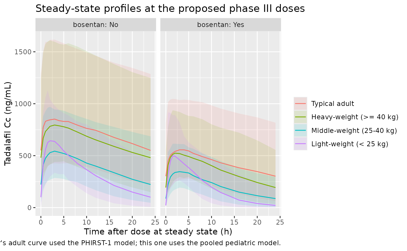
Table 3 was generated by simulating patients at the median weight and age of each cohort, with between-subject variability. The virtual cohort below does the same: 200 patients in each of the eight cohort x bosentan groups, at the proposed phase III doses (40 mg for adults and heavy-weight children, 20 mg for middle- and light-weight children), dosed once daily to steady state.
# rxode2's simulation RNG is partitioned per solver thread, so the cohort
# differs between machines; the assertions below are written to hold for any
# cohort (see the comments on each bound).
rxode2::rxSetSeed(20220211)

n_per_group <- 200L
obs_times <- c(0, 0.5, 1, 1.5, 2, 3, 4, 5, 6, 8, 10, 12, 16, 20, 24)

groups <- tidyr::crossing(cohorts, bosentan = c("No", "Yes")) |>
  dplyr::mutate(
    CONMED_BOSENTAN = as.integer(bosentan == "Yes"),
    treatment = paste0(cohort, ", bosentan: ", bosentan),
    group = dplyr::row_number()
  )

make_cohort <- function(g) {
  ids <- (g$group - 1L) * n_per_group + seq_len(n_per_group)
  subj <- tibble::tibble(
    id = ids, WT = g$WT, AGE = g$AGE, DOSE = g$DOSE,
    CONMED_BOSENTAN = g$CONMED_BOSENTAN, dose_mg = g$DOSE,
    cohort = g$cohort, bosentan = g$bosentan, treatment = g$treatment
  )
  dose <- subj |>
    dplyr::mutate(
      time = 0, evid = 1L, amt = DOSE, cmt = "depot", ii = 24, ss = 1L
    )
  obs <- tidyr::crossing(subj, time = obs_times) |>
    dplyr::mutate(evid = 0L, amt = 0, cmt = "central", ii = 0, ss = 0L)
  dplyr::bind_rows(dose, obs)
}

events <- lapply(seq_len(nrow(groups)), function(i) make_cohort(groups[i, ])) |>
  dplyr::bind_rows() |>
  dplyr::arrange(id, time, dplyr::desc(evid)) |>
  # The event columns must precede the DOSE covariate: when a column named
  # DOSE comes before `amt`, rxode2 reads it as the dose-amount column and the
  # covariate is then reported missing ("required for solving: DOSE").
  dplyr::relocate(id, time, evid, amt, cmt, ii, ss) |>
  as.data.frame()

stopifnot(!anyDuplicated(unique(events[, c("id", "time", "evid")])))
Simulation
sim <- rxode2::rxSolve(
  mod,
  events = events,
  # `dose_mg` is a copy of the DOSE covariate: naming a model covariate in
  # `keep` removes it from the solve.
  keep = c("cohort", "bosentan", "treatment", "dose_mg"),
  maxsteps = 1e6
) |>
  as.data.frame() |>
  dplyr::mutate(cohort = factor(cohort, levels = cohort_levels))
#> ℹ parameter labels from comments will be replaced by 'label()'
Replicate published figures
Figure 3: steady-state AUC by cohort
auc_ind <- sim |>
  dplyr::distinct(id, cohort, bosentan, dose_mg, cl, fdepot) |>
  dplyr::mutate(aucss = 1000 * dose_mg * fdepot / cl)

ggplot(auc_ind, aes(cohort, aucss)) +
  geom_boxplot(outlier.shape = NA, coef = 0) +
  facet_wrap(~bosentan, labeller = label_both) +
  coord_cartesian(ylim = c(0, 40000)) +
  labs(
    x = NULL, y = "AUCss (ng*h/mL)",
    title = "Steady-state AUC at the proposed phase III doses",
    caption = paste(
      "Replicates the pediatric-model boxes of Figure 3 of Ferguson-Sells 2022",
      "(40 mg adults and heavy-weight, 20 mg middle- and light-weight)."
    )
  ) +
  theme(axis.text.x = element_text(angle = 30, hjust = 1))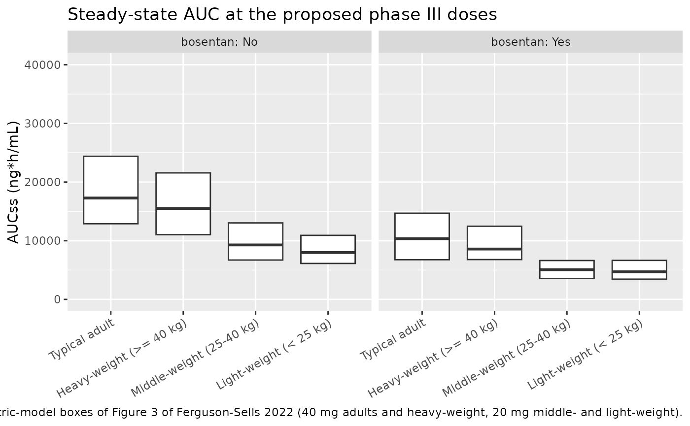
Figure 4a: steady-state concentration-time profiles
sim |>
  dplyr::filter(!is.na(Cc)) |>
  dplyr::group_by(time, cohort, bosentan) |>
  dplyr::summarise(
    Q05 = quantile(Cc, 0.05), Q50 = median(Cc), Q95 = quantile(Cc, 0.95),
    .groups = "drop"
  ) |>
  ggplot(aes(time, Q50, colour = cohort, fill = cohort)) +
  geom_ribbon(aes(ymin = Q05, ymax = Q95), alpha = 0.12, colour = NA) +
  geom_line() +
  facet_wrap(~bosentan, labeller = label_both) +
  labs(
    x = "Time after dose at steady state (h)", y = "Tadalafil Cc (ng/mL)",
    colour = NULL, fill = NULL,
    title = "Steady-state profiles at the proposed phase III doses",
    caption = paste(
      "Replicates Figure 4a of Ferguson-Sells 2022 (median and 90% prediction",
      "interval). The paper's adult curve used the PHIRST-1 model; this one",
      "uses the pooled pediatric model."
    )
  )
PKNCA validation
sim_nca <- sim |>
  dplyr::filter(!is.na(Cc)) |>
  dplyr::select(id, time, Cc, treatment)

conc_obj <- PKNCA::PKNCAconc(
  sim_nca, Cc ~ time | treatment + id,
  concu = "ng/mL", timeu = "h"
)
dose_df <- events |>
  dplyr::filter(evid == 1) |>
  dplyr::select(id, time, amt, treatment)
dose_obj <- PKNCA::PKNCAdose(dose_df, amt ~ time | treatment + id, doseu = "mg")

intervals <- data.frame(
  start = 0, end = 24,
  cmax = TRUE, tmax = TRUE, auclast = TRUE, cav = TRUE
)
nca_res <- PKNCA::pk.nca(PKNCA::PKNCAdata(conc_obj, dose_obj, intervals = intervals))
Comparison against Table 3
published <- table3 |>
  dplyr::mutate(treatment = paste0(cohort, ", bosentan: ", bosentan)) |>
  dplyr::transmute(treatment, auclast = auc, cav = cmean)

cmp <- nlmixr2lib::ncaComparisonTable(
  simulated = nca_res,
  reference = published,
  by = "treatment",
  units = c(auclast = "ng*h/mL", cav = "ng/mL"),
  tolerance_pct = 20
)
knitr::kable(
  cmp,
  caption = paste(
    "Simulated (PKNCA, median) vs. Table 3 AUCtau and Cmean,ss.",
    "* differs from reference by >20%."
  )
)| NCA parameter | treatment | Reference | Simulated | % diff |
|---|---|---|---|---|
| AUClast (ng*h/mL) | Typical adult, bosentan: No | 17100 | 17300 | +1.0% |
| AUClast (ng*h/mL) | Heavy-weight (>= 40 kg), bosentan: No | 15200 | 15400 | +1.5% |
| AUClast (ng*h/mL) | Middle-weight (25-40 kg), bosentan: No | 8390 | 9270 | +10.5% |
| AUClast (ng*h/mL) | Light-weight (< 25 kg), bosentan: No | 8170 | 7960 | -2.6% |
| AUClast (ng*h/mL) | Typical adult, bosentan: Yes | 9870 | 10300 | +4.5% |
| AUClast (ng*h/mL) | Heavy-weight (>= 40 kg), bosentan: Yes | 8990 | 8570 | -4.7% |
| AUClast (ng*h/mL) | Middle-weight (25-40 kg), bosentan: Yes | 5000 | 5050 | +0.9% |
| AUClast (ng*h/mL) | Light-weight (< 25 kg), bosentan: Yes | 4550 | 4680 | +2.9% |
| Cavg (ng/mL) | Typical adult, bosentan: No | 714 | 719 | +0.8% |
| Cavg (ng/mL) | Heavy-weight (>= 40 kg), bosentan: No | 633 | 643 | +1.5% |
| Cavg (ng/mL) | Middle-weight (25-40 kg), bosentan: No | 350 | 386 | +10.3% |
| Cavg (ng/mL) | Light-weight (< 25 kg), bosentan: No | 340 | 332 | -2.4% |
| Cavg (ng/mL) | Typical adult, bosentan: Yes | 411 | 430 | +4.5% |
| Cavg (ng/mL) | Heavy-weight (>= 40 kg), bosentan: Yes | 375 | 357 | -4.8% |
| Cavg (ng/mL) | Middle-weight (25-40 kg), bosentan: Yes | 209 | 210 | +0.6% |
| Cavg (ng/mL) | Light-weight (< 25 kg), bosentan: Yes | 190 | 195 | +2.7% |
auc_chk <- as.data.frame(nca_res$result) |>
  dplyr::filter(PPTESTCD == "auclast") |>
  dplyr::group_by(treatment) |>
  dplyr::summarise(auc_sim = median(PPORRES), .groups = "drop") |>
  dplyr::inner_join(published, by = "treatment") |>
  dplyr::mutate(pct_diff = 100 * (auc_sim / auclast - 1))
stopifnot(nrow(auc_chk) == 8L)
# The simulated AUC median has a Monte Carlo SE of about 4% with 200
# patients per group (CL/F IIV 48.5% CV). A mis-transcribed clearance,
# bioavailability exponent or unit moves every group by tens of percent.
stopifnot(
  abs(median(auc_chk$pct_diff)) < 8,
  max(abs(auc_chk$pct_diff)) < 20
)
The model half-life, log(2) * V / CL, is computed per
patient as Table 3 does (footnote g), rather than from the steady-state
NCA:
thalf_chk <- sim |>
  dplyr::distinct(id, cohort, bosentan, cl, vc) |>
  dplyr::group_by(bosentan, cohort) |>
  dplyr::summarise(
    thalf_sim = median(log(2) * vc / cl),
    q05 = quantile(log(2) * vc / cl, 0.05),
    q95 = quantile(log(2) * vc / cl, 0.95),
    .groups = "drop"
  ) |>
  dplyr::inner_join(table3 |> dplyr::mutate(cohort = factor(cohort, levels = cohort_levels)),
                    by = c("bosentan", "cohort")) |>
  dplyr::mutate(pct_diff = 100 * (thalf_sim / thalf - 1))

thalf_chk |>
  dplyr::transmute(bosentan, cohort,
                   thalf_sim = signif(thalf_sim, 3),
                   pi90 = sprintf("%.3g-%.3g", q05, q95),
                   thalf, pct_diff = round(pct_diff, 1)) |>
  dplyr::rename("Bosentan" = bosentan, "Cohort" = cohort,
                "Simulated median t1/2 (h)" = thalf_sim,
                "Simulated 90% PI (h)" = pi90,
                "Table 3 t1/2 (h)" = thalf, "% diff" = pct_diff) |>
knitr::kable(caption = "Median half-life vs. Table 3.")| Bosentan | Cohort | Simulated median t1/2 (h) | Simulated 90% PI (h) | Table 3 t1/2 (h) | % diff |
|---|---|---|---|---|---|
| No | Typical adult | 29.40 | 13.3-82.5 | 32.00 | -8.1 |
| No | Heavy-weight (>= 40 kg) | 21.90 | 9.65-55.9 | 22.60 | -3.3 |
| No | Middle-weight (25-40 kg) | 14.50 | 6.32-39.9 | 13.50 | 7.5 |
| No | Light-weight (< 25 kg) | 6.67 | 2.84-16.9 | 6.94 | -3.9 |
| Yes | Typical adult | 19.20 | 6.62-52.1 | 18.50 | 3.6 |
| Yes | Heavy-weight (>= 40 kg) | 13.00 | 5.28-32.8 | 13.30 | -2.6 |
| Yes | Middle-weight (25-40 kg) | 8.36 | 3.19-19.9 | 8.08 | 3.5 |
| Yes | Light-weight (< 25 kg) | 4.00 | 1.76-10.1 | 3.78 | 5.8 |
Assumptions and deviations
-
Residual error. Table 2 footnote f reports the
proportional error as
100% * sqrt(sigma1)and the additive error assqrt(x^2 * sigma1), wherexis the additive-error THETA andsigma1the single residual variance. That is one epsilon scaled bysqrt(IPRED^2 + x^2), i.e. a residual variance ofpropSd^2 * IPRED^2 + addSd^2, which is how nlmixr2 combinesadd(addSd) + prop(propSd)by default. The model uses the point estimateaddSd = 11.6ng/mL. The bootstrap column of Table 2 prints 43.3 ng/mL (17.4, 70.0) for the same row, whose interval does not contain 11.6. The bootstrap value matches the raw THETAxinstead:11.6 / 0.258 = 45.0, so the maintainers read the bootstrap column as reportingxunconverted, and took the SD from the point-estimate column. -
Bosentan reference category. The paper’s typical
CL/F (3.23 L/h) is for patients taking bosentan and the estimated
coefficient (-0.418) is the change for patients not taking it. The
canonical
CONMED_BOSENTANcolumn keeps its 1 = bosentan coding, and the coefficient is applied to(1 - CONMED_BOSENTAN), so the published values are used unchanged. Ambrisentan users takeCONMED_BOSENTAN = 0, as in the paper. -
Dose and age covariates.
DOSEis the administered dose in mg on each record and may change within a patient (the pediatric study stepped from a low to a high dose).AGEis age at study entry. The centring values 16.27 mg and 52.4 years are printed in the Table 2 equation; the paper does not say how they were chosen. - Table 3 adult rows. Table 3 also lists typical adults under the earlier PHIRST-1 adult-only model (CL/F 2.46 and 4.31 L/h). That model is a different model (not published in full) and is not reproduced here; only the pooled pediatric-model rows are compared.
- Extrapolation. No patient under 2 years was enrolled and the paper warns the model should not be extrapolated to younger children, because the CYP3A7-to-CYP3A4 switch in infancy is not described by the model.
- No erratum or correction notice was found for this article (Europe PMC search, 2026-09-30).