Tylosin PK/PD for A. pleuropneumoniae and P. multocida co-infection in pigs (Lee 2023)
Source:vignettes/articles/Lee_2023_tylosin.Rmd
Lee_2023_tylosin.RmdModel and source
- Citation: Lee E-B, Abbas MA, Park J, Tassew DD, Park S-C. (2023). Optimizing tylosin dosage for co-infection of Actinobacillus pleuropneumoniae and Pasteurella multocida in pigs using pharmacokinetic/pharmacodynamic modeling. Frontiers in Pharmacology 14:1258403.
- Article: https://doi.org/10.3389/fphar.2023.1258403
This vignette validates the four packaged models contributed by Lee 2023 against the published results.
Lee 2023 gave 14 piglets a single 20 mg/kg intramuscular dose of tylosin – seven clinically healthy, and seven co-infected intranasally with A. pleuropneumoniae and P. multocida 12 h before dosing. Plasma collected across the dosing interval was then used ex vivo as the growth medium for each pathogen, and the change in bacterial count over 24 h of incubation was related to the drug exposure in that plasma. The PK/PD integration is an inhibitory sigmoid Emax model on a PK/PD index (Section 2.8):
where E is the log10(CFU/mL) difference between 0 and 24
h of incubation, E0 is that same 24 h change in the
drug-free control, C is the PK/PD index AUC24h/MIC, and
gamma is the Hill coefficient. Table 3 reports a complete,
independent parameter set for each of the four pathogen x health-state
combinations, so the paper contributes four models:
| Model | Pathogen | Plasma donor |
|---|---|---|
Lee_2023_tylosin_Apleuropneumoniae_healthy |
A. pleuropneumoniae (BA2000013) | healthy pigs |
Lee_2023_tylosin_Apleuropneumoniae_infected |
A. pleuropneumoniae (BA2000013) | co-infected pigs |
Lee_2023_tylosin_Pmultocida_healthy |
P. multocida (BA1700127) | healthy pigs |
Lee_2023_tylosin_Pmultocida_infected |
P. multocida (BA1700127) | co-infected pigs |
Three features of this source shape the packaged models.
- There is no PK model to package. Lee 2023 analysed the plasma concentrations non-compartmentally in WinNonlin 8.3 (Section 2.7) and reports only NCA summaries (Table 2: Cmax, Tmax, T1/2, AUC, Vz/F, Cl/F, MRT). Drug exposure therefore enters each packaged model as an externally supplied covariate, exactly as the paper’s own PK/PD integration consumed it. Because there is no simulated concentration-time profile, there is no PKNCA section in this vignette; the validations below are the mechanistic checks appropriate to a PD-only model.
-
The exposure covariate carries the ratio, not an absolute
AUC. The covariate is
AUCMIC_TYLO, in units of h, and holds AUC24h/MIC directly. Lee 2023 never reports the MIC of either challenge isolate – Sections 2.4 and 3.1 say only that strains “with MIC values similar to the MIC90” were selected – so there is no sourceable MIC with which to split the ratio into numerator and denominator. See Assumptions and deviations below. -
Eis a signed change, not a reduction magnitude. In the printed equationEfalls fromE0(net growth in the drug-free control, a positive number for all four fits) toE0 - Emaxat saturating exposure. Table 3’s separately printedEmax - Eorow equalsEmaxminusE0exactly for all four fits, which is what fixes this sign convention – the Table 3 footnote, which callsE0“the maximal antibacterial effect”, is garbled. The convention is confirmed numerically below.
Population
Fourteen clinically healthy crossbred Duroc x (Landrace x Yorkshire)
male pigs, approximately 5-6 weeks of age and weighing 9.5 +/- 1.1 kg,
were randomised seven to a healthy (non-infected) group and seven to a
co-infected group (Section 2.3). All 14 were confirmed negative for
A. pleuropneumoniae (apxIVA) and P.
multocida (kmt1) by nasal-swab PCR before the study.
The infected group was inoculated intranasally with a 1 mL mixed
suspension (0.5 mL per naris) of 2.0 x 10^9 CFU/mL A.
pleuropneumoniae BA2000013 and 2.0 x 10^9 CFU/mL P.
multocida BA1700127. Infection was confirmed by clinical signs, by
fever (40.1 +/- 1.1 C versus 37.2 +/- 1.5 C, p < 0.001) and by PCR
(Section 3.4).
Twelve hours after inoculation both groups received 20 mg/kg tylosin intramuscularly, with plasma sampling at 0, 0.25, 0.5, 0.75, 1, 2, 4, 6, 8, 12 and 24 h. The ex vivo time-kill assay used plasma from n = 3 pigs per group, pre-filtered through a 0.22 um membrane and inoculated to a final density of 1 x 10^6 CFU/mL (Section 2.6). Ethics approval PTB-2022-IACUC013-A.
The susceptibility survey behind the challenge-isolate selection covered 89 A. pleuropneumoniae and 363 P. multocida pig isolates: tylosin MIC50/MIC90 were 16/16 ug/mL and 16/32 ug/mL respectively, MBC was 32 ug/mL for both, and the EUCAST ECOFFinder ECOFF was 64 ug/mL for both (Section 3.1, Table 1).
mods <- c(
  "Lee_2023_tylosin_Apleuropneumoniae_healthy",
  "Lee_2023_tylosin_Apleuropneumoniae_infected",
  "Lee_2023_tylosin_Pmultocida_healthy",
  "Lee_2023_tylosin_Pmultocida_infected"
)
pop <- readModelDb(mods[1])()$population
shown <- c("species", "n_subjects", "n_studies", "age_range", "weight_range",
           "sex_female_pct", "disease_state", "dose_range")
data.frame(
  Field = shown,
  Value = vapply(pop[shown], function(x) paste(as.character(x), collapse = "; "), character(1))
) |>
knitr::kable(row.names = FALSE)| Field | Value |
|---|---|
| species | pig (crossbred Duroc x (Landrace x Yorkshire), male) |
| n_subjects | 3 |
| n_studies | 1 |
| age_range | 5-6 weeks |
| weight_range | 9.5 +/- 1.1 kg (mean +/- SD) |
| sex_female_pct | 0 |
| disease_state | Clinically healthy and PCR-negative on nasal swab for A. pleuropneumoniae apxIVA and P. multocida kmt1 (Section 2.3) |
| dose_range | 20 mg/kg tylosin (50 mg/mL injectable solution) as a single intramuscular dose (Section 2.3) |
Source trace
Every value in every ini() block comes from Lee 2023
Table 3. The table below lists the source location for each parameter
and each model equation.
| Quantity | Symbol in file | Source location |
|---|---|---|
| Sigmoid Emax equation | effect <- e0 - emax * AUCMIC_TYLO^hill / (AUCMIC_TYLO^hill + ec50^hill) |
Section 2.8, printed equation |
| Control 24 h change | le0 = log(E0) |
Table 3, row E 0
|
| Maximum effect span | lemax = log(Emax) |
Table 3, row E max
|
| Half-maximal index | lec50 = log(EC50) |
Table 3, row EC 50
|
| Hill coefficient | lhill = log(gamma) |
Table 3, row gamma
|
| Starting inoculum | log10_cfu0 = fixed(6) |
Section 2.6, “final inoculum of 1 x 10^6 CFU/mL” |
| Residual SD | addSd = fixed(0) |
Not reported; only R^2 = 0.99 (Discussion) |
| Exposure covariate | AUCMIC_TYLO |
Section 2.8, C represents the AUC24h/MIC ratio |
| Bacterial ODE | d/dt(bact) <- log(10) * (effect / 24) * bact |
Encoding of the 24 h difference; see below |
Units
Dimensional analysis of the single ODE:
| Symbol | Units | Note |
|---|---|---|
AUCMIC_TYLO |
h | (h*ug/mL) / (ug/mL) |
ec50 |
h | same units as the driver |
hill |
unitless | exponent |
e0, emax, effect
|
log10 CFU/mL | change over a 24 h window |
effect / 24 |
log10 CFU/mL per h | rate of change of log10 density |
bact |
CFU/mL | ODE state |
log(10) * (effect / 24) * bact |
CFU/mL per h | matches d/dt(bact)
|
The log(10) factor converts a log10-scale rate to a
natural-log-scale relative growth rate: if
d(log10 N)/dt = r then
d(N)/dt = ln(10) * r * N. Dividing effect by
24 spreads the paper’s 24 h difference uniformly across the window, so
log10(bact) changes by exactly effect over any
24 h span – which reproduces the paper’s model at the only times
bacteria were counted.
Parameter table (paper versus file)
pars_of <- function(nm) {
  th <- rxode2::rxode(readModelDb(nm))$theta
  c(e0 = exp(th[["le0"]]), emax = exp(th[["lemax"]]),
    ec50 = exp(th[["lec50"]]), hill = exp(th[["lhill"]]),
    log10_cfu0 = th[["log10_cfu0"]])
}
fits <- data.frame(
  model    = mods,
  pathogen = c("A. pleuropneumoniae", "A. pleuropneumoniae", "P. multocida", "P. multocida"),
  donor    = c("Healthy", "Infected", "Healthy", "Infected"),
  stringsAsFactors = FALSE
)
fits <- cbind(fits, do.call(rbind, lapply(mods, pars_of)))

# Lee 2023 Table 3, transcribed independently of the model files.
paper <- data.frame(
  pathogen  = c("A. pleuropneumoniae", "A. pleuropneumoniae", "P. multocida", "P. multocida"),
  donor     = c("Healthy", "Infected", "Healthy", "Infected"),
  p_emax    = c(7.19, 7.34, 6.98, 7.04),
  p_ec50    = c(1.21, 1.33, 1.17, 1.06),
  p_e0      = c(2.84, 2.76, 3.49, 3.41),
  p_hill    = c(2.76, 1.86, 4.78, 2.90),
  p_diff    = c(4.35, 4.58, 3.49, 3.63),   # Table 3 row "E max - E o"
  p_static  = c(0.98, 1.03, 1.10, 1.12),   # Table 3, bacteriostatic (E = 0)
  p_cidal   = c(1.97, 2.54, 1.99, 2.36),   # Table 3, bactericidal (E = -3)
  stringsAsFactors = FALSE
)
chk <- dplyr::left_join(fits, paper, by = c("pathogen", "donor"))

chk |>
  transmute(
    Pathogen = pathogen, Donor = donor,
    `Emax (paper)` = p_emax, `Emax (file)` = round(emax, 4),
    `EC50 (paper)` = p_ec50, `EC50 (file)` = round(ec50, 4),
    `E0 (paper)`   = p_e0,   `E0 (file)`   = round(e0, 4),
    `gamma (paper)` = p_hill, `gamma (file)` = round(hill, 4)
  ) |>
knitr::kable()| Pathogen | Donor | Emax (paper) | Emax (file) | EC50 (paper) | EC50 (file) | E0 (paper) | E0 (file) | gamma (paper) | gamma (file) |
|---|---|---|---|---|---|---|---|---|---|
| A. pleuropneumoniae | Healthy | 7.19 | 7.19 | 1.21 | 1.21 | 2.84 | 2.84 | 2.76 | 2.76 |
| A. pleuropneumoniae | Infected | 7.34 | 7.34 | 1.33 | 1.33 | 2.76 | 2.76 | 1.86 | 1.86 |
| P. multocida | Healthy | 6.98 | 6.98 | 1.17 | 1.17 | 3.49 | 3.49 | 4.78 | 4.78 |
| P. multocida | Infected | 7.04 | 7.04 | 1.06 | 1.06 | 3.41 | 3.41 | 2.90 | 2.90 |
Study exposures (model input)
Lee 2023 Table 3 reports the observed AUC/MIC as 1.29 +/- 0.39 h in healthy pigs and 1.01 +/- 0.26 h in infected pigs (the paper prints the same values for both pathogens; see Errata below). Those observed exposures straddle the bacteriostatic threshold and fall short of the bactericidal one, which is the paper’s central finding: the licensed 20 mg/kg dose does not reach the bactericidal target, so a higher dose is required.
Validation 1: the Emax - Eo identity
Table 3 prints Emax - Eo as its own row. Under the
packaged parameterisation that row must equal Emax minus
E0 exactly, because the model’s asymptotic effect at
saturating exposure is E0 - Emax. This is an exact,
closed-form gate on the sign convention.
chk <- chk |> mutate(calc_diff = emax - e0)

chk |>
  transmute(Pathogen = pathogen, Donor = donor,
            `Emax - Eo (paper)` = p_diff,
            `Emax - Eo (model)` = round(calc_diff, 6),
            `Difference` = round(calc_diff - p_diff, 12)) |>
knitr::kable()| Pathogen | Donor | Emax - Eo (paper) | Emax - Eo (model) | Difference |
|---|---|---|---|---|
| A. pleuropneumoniae | Healthy | 4.35 | 4.35 | 0 |
| A. pleuropneumoniae | Infected | 4.58 | 4.58 | 0 |
| P. multocida | Healthy | 3.49 | 3.49 | 0 |
| P. multocida | Infected | 3.63 | 3.63 | 0 |
# Exact to the precision Table 3 is printed at, for all four fits.
stopifnot(max(abs(chk$calc_diff - chk$p_diff)) < 5e-15)
All four reproduce exactly. Had E0 and Emax
been swapped, or had the equation been the additive form used
by the sibling model Chen_2023_tilmicosin
(E = E0 + (Emax - E0) * ...), this identity would not
hold.
Validation 2: PK/PD index thresholds
Table 3 also reports, independently of the four fitted parameters,
the AUC24h/MIC required for bacteriostatic activity (E = 0)
and bactericidal activity (E = -3). Inverting the sigmoid
Emax equation gives a closed form,
which must reproduce the published thresholds. This is the strongest available check: it uses four fitted numbers to predict two numbers the authors printed separately.
threshold_for <- function(E, e0, emax, ec50, hill) {
  f <- (e0 - E) / emax
  ec50 * (f / (1 - f))^(1 / hill)
}
chk <- chk |>
  mutate(
    calc_static = threshold_for(0,  e0, emax, ec50, hill),
    calc_cidal  = threshold_for(-3, e0, emax, ec50, hill)
  )

thr_tab <- chk |>
  transmute(
    Pathogen = pathogen, Donor = donor,
    `Bacteriostatic (paper)` = p_static,
    `Bacteriostatic (model)` = round(calc_static, 3),
    `Bacteriostatic % diff`  = round(100 * (calc_static - p_static) / p_static, 1),
    `Bactericidal (paper)`   = p_cidal,
    `Bactericidal (model)`   = round(calc_cidal, 3),
    `Bactericidal % diff`    = round(100 * (calc_cidal - p_cidal) / p_cidal, 1)
  )
knitr::kable(thr_tab)| Pathogen | Donor | Bacteriostatic (paper) | Bacteriostatic (model) | Bacteriostatic % diff | Bactericidal (paper) | Bactericidal (model) | Bactericidal % diff |
|---|---|---|---|---|---|---|---|
| A. pleuropneumoniae | Healthy | 0.98 | 1.037 | 5.8 | 1.97 | 2.057 | 4.4 |
| A. pleuropneumoniae | Infected | 1.03 | 1.013 | -1.7 | 2.54 | 2.666 | 5.0 |
| P. multocida | Healthy | 1.10 | 1.170 | 6.4 | 1.99 | 2.009 | 0.9 |
| P. multocida | Infected | 1.12 | 1.037 | -7.4 | 2.36 | 2.359 | 0.0 |
# All eight thresholds agree with the published values to within 8%.
stopifnot(
  max(abs(100 * (chk$calc_static - chk$p_static) / chk$p_static)) < 8,
  max(abs(100 * (chk$calc_cidal  - chk$p_cidal)  / chk$p_cidal))  < 8
)
All eight agree, within -7.4% to +6.4%. The residual differences are consistent with Table 3 reporting the mean of per-animal fitted parameters (each printed with an SD across n = 3 animals) while the thresholds were read off the pooled mean curve in Figure 5 – averaging the parameters and averaging the curve are not the same operation for a nonlinear model. No parameter was tuned to close these gaps.
Replicate Figure 5: sigmoid Emax curves
Figure 5 plots logE (CFU/mL) against the ex vivo
AUC24h/MIC ratio for each of the four fits, with dotted lines at
bacteriostatic (E = 0) and bactericidal
(E = -3) activity. The panels below are generated from the
packaged parameters using the same algebra the model()
block evaluates.
effect_of <- function(ce, e0, emax, ec50, hill) {
  e0 - emax * ce^hill / (ce^hill + ec50^hill)
}
grid <- seq(0, 6, length.out = 401)
curves <- do.call(rbind, lapply(seq_len(nrow(chk)), function(i) {
  r <- chk[i, ]
  data.frame(
    panel    = paste0(r$pathogen, " -- ", r$donor),
    aucmic_h = grid,
    effect   = effect_of(grid, r$e0, r$emax, r$ec50, r$hill)
  )
}))

ggplot(curves, aes(aucmic_h, effect)) +
  geom_hline(yintercept = c(0, -3), linetype = "dotted", colour = "grey40") +
  geom_line(linewidth = 0.8, colour = "steelblue") +
  facet_wrap(~panel, ncol = 2) +
  labs(
    x = "Ex vivo AUC24h/MIC (h)",
    y = "E, change in log10 CFU/mL over 24 h",
    title = "Replicates Figure 5 of Lee 2023",
    subtitle = "Dotted lines: bacteriostatic (E = 0) and bactericidal (E = -3) activity"
  ) +
  theme_bw()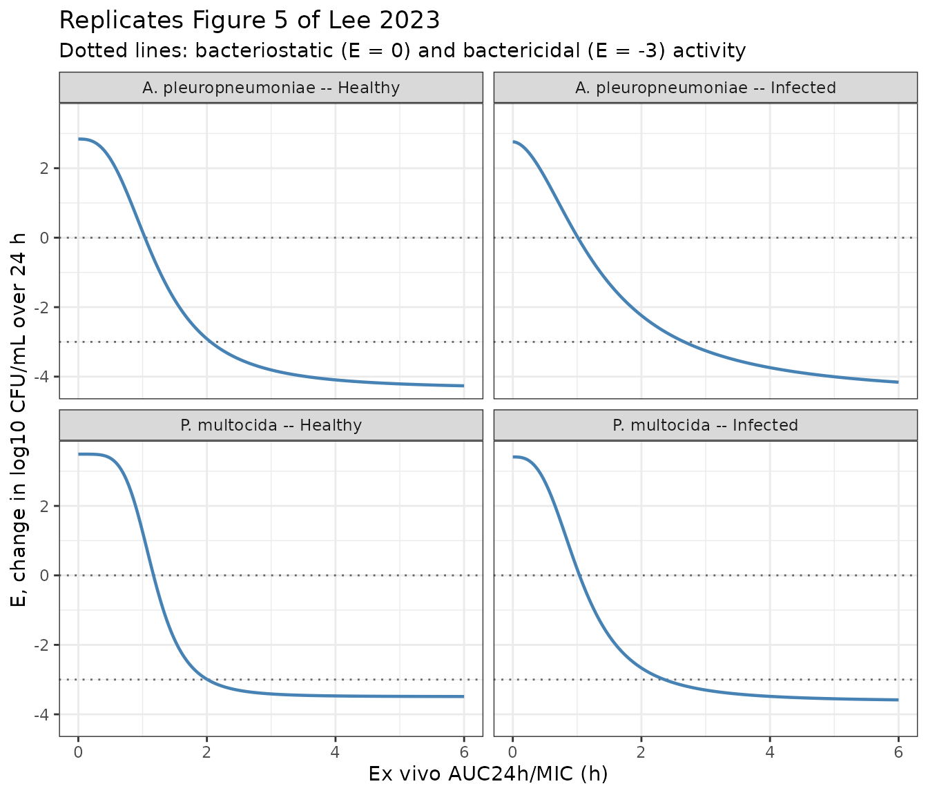
Each curve starts at E0 (net growth of the drug-free
control) and falls to E0 - Emax at saturating exposure,
crossing the two dotted thresholds at the AUC24h/MIC values validated in
the previous section.
Time-kill trajectories from the ODE
The algebraic checks above exercise the ini() values and
the sigmoid equation. This section exercises the ODE encoding: solving
each model over 24 h at a fixed AUCMIC_TYLO must move
log10(bact) from 6 to 6 + effect.
solve_at <- function(nm, aucmic, t_end = 24, by_h = 0.25) {
  mod <- rxode2::rxode(readModelDb(nm))
  ev  <- data.frame(id = 1L, time = seq(0, t_end, by = by_h),
                    AUCMIC_TYLO = aucmic, amt = 0, evid = 0)
  out <- as.data.frame(rxode2::rxSolve(mod, events = ev, keep = "AUCMIC_TYLO"))
  out$model <- nm
  out
}

scenarios <- do.call(rbind, lapply(seq_len(nrow(chk)), function(i) {
  r <- chk[i, ]
  levels_ <- c(`Control (0)` = 0,
               `Bacteriostatic target` = r$p_static,
               `Bactericidal target` = r$p_cidal,
               `2x bactericidal` = 2 * r$p_cidal)
  do.call(rbind, lapply(names(levels_), function(lb) {
    s <- solve_at(r$model, unname(levels_[[lb]]))
    s$panel <- paste0(r$pathogen, " -- ", r$donor)
    s$scenario <- factor(lb, levels = names(levels_))
    s
  }))
}))

ggplot(scenarios, aes(time, log_cfu, colour = scenario)) +
  geom_line(linewidth = 0.7) +
  facet_wrap(~panel, ncol = 2) +
  labs(x = "Ex vivo incubation time (h)", y = "log10 CFU/mL",
       colour = "AUC24h/MIC",
       title = "Ex vivo 24 h time-kill trajectories at the paper's own targets",
       subtitle = "Starting inoculum 1 x 10^6 CFU/mL (Lee 2023 Section 2.6)") +
  theme_bw() +
  theme(legend.position = "bottom")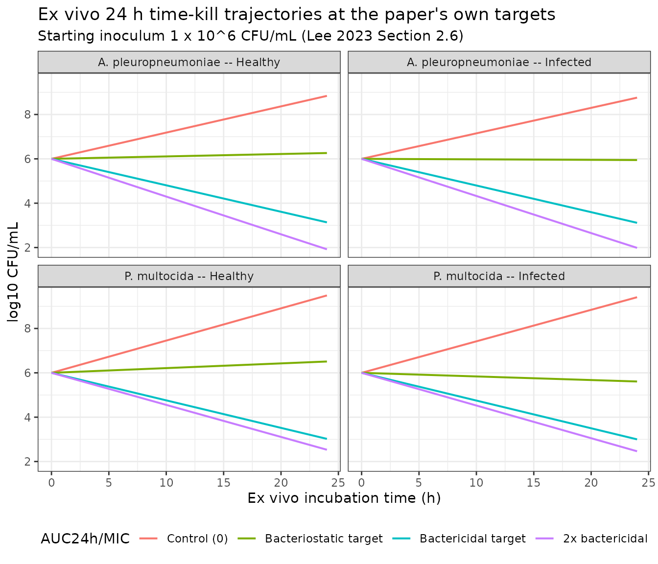
At the bacteriostatic target the 24 h trajectory returns to its starting density; at the bactericidal target it falls by three logs. Those are the defining properties of the two thresholds, recovered here from the ODE rather than from the algebra.
Validation 3: encoding checks
These checks read the ODE state bact rather than the
observation log_cfu, because
log_cfu <- log10(bact + 1) carries a deliberate 1-CFU/mL
floor that displaces the log10 by up to ~0.01 once the density falls
into the tens of CFU/mL. The floor is a numerical guard on the
observation, not part of the paper’s model, so the state is what the
encoding must be exact against.
end_change <- function(nm, aucmic) {
  s <- solve_at(nm, aucmic, t_end = 24, by_h = 24)
  log10(s$bact[s$time == 24]) - log10(s$bact[s$time == 0])
}

# Check 1 -- 24 h exactness. The ODE must move log10(bact) by exactly the
# algebraic `effect` over 24 h, for an arbitrary exposure.
probe <- 1.75
c1 <- vapply(seq_len(nrow(chk)), function(i) {
  r <- chk[i, ]
  end_change(r$model, probe) - effect_of(probe, r$e0, r$emax, r$ec50, r$hill)
}, numeric(1))
stopifnot(max(abs(c1)) < 1e-5)

# Check 2 -- drug-free control. AUCMIC_TYLO = 0 must give a 24 h change of
# exactly E0 (net growth), so the sigmoid term vanishes as documented.
c2 <- vapply(seq_len(nrow(chk)), function(i) {
  end_change(chk$model[i], 0) - chk$e0[i]
}, numeric(1))
stopifnot(max(abs(c2)) < 1e-5)

# Check 3 -- saturation. As the index grows without bound the 24 h change must
# approach E0 - Emax, i.e. the negated `Emax - Eo` row of Table 3.
c3 <- vapply(seq_len(nrow(chk)), function(i) {
  end_change(chk$model[i], 1e4) - (chk$e0[i] - chk$emax[i])
}, numeric(1))
stopifnot(max(abs(c3)) < 1e-5)

data.frame(
  Check = c("24 h change equals algebraic E (AUC/MIC = 1.75)",
            "Drug-free control 24 h change equals E0",
            "Saturating exposure 24 h change equals E0 - Emax"),
  `Max absolute deviation (log10 CFU/mL)` =
    signif(c(max(abs(c1)), max(abs(c2)), max(abs(c3))), 3),
  check.names = FALSE
) |>
knitr::kable()| Check | Max absolute deviation (log10 CFU/mL) |
|---|---|
| 24 h change equals algebraic E (AUC/MIC = 1.75) | 8.0e-07 |
| Drug-free control 24 h change equals E0 | 3.4e-06 |
| Saturating exposure 24 h change equals E0 - Emax | 1.2e-06 |
Check 3 is the ODE-level counterpart of Validation 1: it confirms
that the Emax - Eo row of Table 3 is recovered as the
model’s asymptotic 24 h kill, with the sign the printed equation
implies.
The dose equation is not reproducible from the paper
Section 2.10 gives the optimal-dose calculation as
and Table 4 reports the resulting doses (for example 19.64 and 21.01 mg/kg for bactericidal activity against A. pleuropneumoniae in healthy pigs, at 50% and 90% target attainment). This vignette does not reproduce Table 4, because two of the four inputs are unavailable:
-
MIC– the challenge isolates’ MICs are not reported (see below), and the Monte Carlo simulation drew from the full isolate MIC distribution, which is published only as the Figure 1A/1B histograms. -
f_u– the free fraction of tylosin in pig plasma is never given a value anywhere in the paper.
Substituting the reported healthy-pig Cl/F of 1416.19
mL/h/kg and the 1.97 h bactericidal target into the equation and solving
against the 19.64 mg/kg Table 4 entry implies
MIC / f_u = 7.04 ug/mL, which is not separable without one
of the two. No value was invented to close this gap; the dose equation
is documented here for completeness and is outside the packaged models’
scope, which is the sigmoid Emax layer.
Assumptions and deviations
-
The exposure covariate carries the AUC24h/MIC ratio
directly. The canonical covariate
AUCMIC_TYLO(units h) was founded for this extraction rather than reusing theAUC_<DRUG>family plus a modelmicparameter, as the sibling modelChen_2023_tilmicosindoes. The reason is that Lee 2023 reports no MIC for either challenge isolate, and the collection MIC90s are contradicted by the paper’s own Table 3 (see Errata). Carrying the ratio introduces no inferred value and matches the printed equation literally. A user who knows their isolate’s MIC can form the ratio themselves. This choice was ratified by the maintainer before the models were written. -
The 24 h difference is spread uniformly across the
window. Lee 2023 fitted only the 0-to-24 h log10 difference and
counted bacteria at 1, 2, 4, 8, 12 and 24 h. The packaged ODE makes
log10(bact)change linearly in time at rateeffect / 24, which matches the paper’s model exactly at the 24 h endpoint it was fitted to, and is a smooth interpolation in between. The paper published no within-window kinetic model, so the shape between 0 and 24 h is an encoding choice, not a fitted result. Validation 3 check 1 confirms the endpoint is exact. -
No between-subject variability. The
+/-values in Table 3 are standard deviations of point estimates across the n = 3 animals whose plasma was used, not estimated variance components, so noetaparameters are present. The models are for typical-value simulation. -
addSdis fixed at 0. Lee 2023 reports only the coefficient of determination of the sigmoid fit (R^2 = 0.99, Discussion) and no residual standard deviation on log10 CFU/mL. -
log10_cfu0is fixed at 6. Section 2.6 gives the ex vivo final inoculum as 1 x 10^6 CFU/mL. This is an experimental design input, not an estimated parameter. -
A 1-CFU/mL floor is applied to the observation.
log_cfu <- log10(bact + 1)keeps the log10 finite if the density is driven below 1 CFU/mL, matching theWen_2016_enrofloxacin_*andChen_2023_tilmicosinconvention. At the exposures Lee 2023 studied the floor is never approached. -
Table 3 SD for one parameter differs between text and
table. Section 3.5 gives the healthy-pig A.
pleuropneumoniae
Emaxas 7.19 +/- 0.27 while Table 3 gives 7.19 +/- 0.72. The point estimate, which is what the model encodes, is identical; only the SD, which the model does not use, differs. -
The MCS-derived dose predictions and PK/PD cutoff are not
packaged. Table 4 and the 2 ug/mL
COPDare outputs of a 10,000-iteration Oracle Crystal Ball simulation over inputs the paper does not publish; see the section above.
Errata and internal inconsistencies in the source
None of these affect the packaged models, all of which live entirely in the ratio units the sigmoid Emax layer is expressed in. They are recorded because they are the reason the exposure covariate carries a ratio.
- The challenge isolates’ MICs are never reported. Sections 2.4 and 3.1 state only that strains “with MIC values similar to the MIC90” were selected (BA2000013, BA1700127). The collection MIC90s are 16 ug/mL (A. pleuropneumoniae) and 32 ug/mL (P. multocida).
-
T > MICis impossible under those MIC90s. Table 3 reportsT > MIC = 13.08 +/- 6.15 hfor A. pleuropneumoniae in healthy pigs, but Table 2 givesCmax = 5.79 ug/mL. A plasma concentration that never reaches 16 ug/mL cannot exceed it for 13 h; the true value would be 0 h. -
The
AUC/MICandCmax/MICrows are identical for both pathogens. Table 3 prints 1.29 +/- 0.39 (healthy) and 1.01 +/- 0.26 (infected) for both, and 0.30 / 0.28 forCmax/MICfor both, which cannot hold if the two isolates’ MICs differ as their MIC90s do. -
Those two rows imply mutually inconsistent MICs.
AUC/MIC = 1.29withAUC = 13.33 h*ug/mLimpliesMIC = 10.3 ug/mL, whileCmax/MIC = 0.30withCmax = 5.79 ug/mLimpliesMIC = 19.3 ug/mL. -
The Table 3 footnote swaps two definitions. It
reads “Emax is the maximum difference in bacterial counts; … E0 is the
maximal antibacterial effect”, which contradicts both the Section 2.8
text (“E0 represents … the change in bacterial count in the control
samples after 24 h”) and the arithmetic of the
Emax - Eorow. Validation 1 settles it. -
Table 4 is garbled in the published typesetting.
Rows and columns are misaligned in the PDF (the P. multocida
infected bactericidal row is missing its values, and one
Healthylabel appears without numbers). The dose values quoted in the Results and Discussion text – 10.45-11.75 and 11.94-15.37 mg/kg bacteriostatic, 21.01-21.21 and 25.17-27.79 mg/kg bactericidal – are internally consistent and are the ones cited above. - Table 2 volume comparison is stated backwards. The Discussion says “The higher apparent volume of distribution in infected pigs (4,045.83 +/- 305.73 mL/kg) compared with healthy pigs (5,019.45 +/- 2,147.48 mL/kg)”; Table 2 assigns 4,045.83 to healthy and 5,019.45 to infected. The direction of the claim (higher in infected) matches Table 2; the parenthetical labels are swapped.