Midazolam (van Rongen 2015)
Source:vignettes/articles/vanRongen_2015_midazolam.Rmd
vanRongen_2015_midazolam.RmdModel and source
- Citation: van Rongen A, Vaughns JD, Moorthy GS, Barrett JS, Knibbe CAJ, van den Anker JN (2015). Population pharmacokinetics of midazolam and its metabolites in overweight and obese adolescents. Br J Clin Pharmacol 80(5):1185-1196. doi:10.1111/bcp.12693.
- Description: Joint parent-and-sequential-metabolites population PK model for intravenous midazolam, its primary CYP3A oxidative metabolite 1’-hydroxymidazolam (1-OH-midazolam), and the downstream phase-II 1’-hydroxymidazolam glucuronide (1-OH-midazolam glucuronide) in 19 overweight and obese adolescents (12.5-18.9 years, body weight 62-149.8 kg) undergoing surgery (van Rongen 2015). Two-compartment disposition for midazolam (central + peripheral) routes the entire elimination clearance CL1 to 1-OH-midazolam formation. 1-OH-midazolam is described by a one-compartment model with apparent volume of distribution fixed at 0.9 times the midazolam central volume (Mandema 1992); the entire 1-OH-midazolam clearance CL3 is routed to 1-OH-midazolam glucuronide formation. 1-OH-midazolam glucuronide is described by a two-compartment model with renal elimination clearance CL4. Total body weight (TBW) enters the peripheral volume of distribution of midazolam as a power function with reference 104.7 kg (cohort median) and estimated exponent X = 1.68; no other covariate effect was retained. Concentrations are modeled in umol/L throughout (paper Methods), so dosing is in umol; dose_umol = dose_mg * 1000 / MW_midazolam where MW_midazolam = 325.77 g/mol.
- Article: https://doi.org/10.1111/bcp.12693
Population
The model was fit to 19 overweight and obese adolescents (13 female, 6 male) aged 12.5-18.9 years (mean 15.9 +/- 1.6 years) with body weight 62-149.8 kg (mean 102.7 +/- 24.9 kg) undergoing general surgery (orthopaedics, tonsillectomy, bariatric surgery) at Children’s National Medical Center, Washington DC. Three patients were classified as overweight (BMI for age >=85th percentile) and 16 as obese (>=95th percentile); BMI ranged 24.8-55 kg/m^2 and BMI z-score 1.5-2.7. Demographics are in Table 1 of van Rongen 2015. The cohort median total body weight, 104.7 kg, is the reference used in the power-function TBW effect on the midazolam peripheral volume of distribution (paper Table 2 final model).
Each subject received a single intravenous bolus dose of 2 mg (n = 16) or 3 mg (n = 3) midazolam shortly before transfer to the operating room. Blood samples were drawn at t = 0, (5), 15, 30 min and 1, 2, 4, 6, occasionally 8 h post-dose. The model was estimated on a total of 129 midazolam, 118 1’-hydroxymidazolam, and 128 1’-hydroxymidazolam glucuronide concentrations using NONMEM 7.2 with first-order conditional estimation.
The same information is available programmatically via the model’s
population metadata
(rxode2::rxode(readModelDb("vanRongen_2015_midazolam"))$meta$population).
Source trace
The per-parameter origin is recorded as an in-file comment next to
each ini() entry in
inst/modeldb/specificDrugs/vanRongen_2015_midazolam.R. The
table below collects them in one place for review.
| Equation / parameter | Value | Source location |
|---|---|---|
| Two-compartment midazolam, one-compartment 1-OH-midazolam, two-compartment 1-OH-midazolam glucuronide | n/a | Methods page 1187; Figure 1 page 1189 |
| Concentrations on the umol/L molar scale (MW_mdz = 325.77, MW_1ohm = 341.77, MW_1ohmg = 517.9 g/mol) | n/a | Methods page 1187 |
| V_1-OH-midazolam = 0.9 x V_mdz,central (fixed, structural) | n/a | Methods page 1187 citing Mandema 1992 |
| CL1 (midazolam total clearance) | 0.66 L/min | Table 2 page 1190 final model column |
| V_mdz,central | 39.8 L | Table 2 page 1190 final model column |
| V_mdz,peripheral at TBW = 104.7 kg | 154 L | Table 2 page 1190 final model column |
| TBW power exponent X on V_mdz,peripheral | 1.68 | Table 2 page 1190 final model column |
| Q (midazolam inter-compartmental clearance) | 1.18 L/min | Table 2 page 1190 final model column |
| CL3 (1-OH-midazolam total clearance) | 1.85 L/min | Table 2 page 1190 final model column |
| V_1-OH-midazolam-gluc,central | 4.05 L | Table 2 page 1190 final model column |
| V_1-OH-midazolam-gluc,peripheral | 15.9 L | Table 2 page 1190 final model column |
| Q2 (1-OH-midazolam-gluc inter-compartmental clearance) | 0.49 L/min | Table 2 page 1190 final model column |
| CL4 (1-OH-midazolam-gluc elimination) | 0.42 L/min | Table 2 page 1190 final model column |
| IIV CL1 (CV%) | 23.7 | Table 2 page 1190 final model column |
| IIV V_mdz,central = V_1-OH (CV%) | 30.5 | Table 2 page 1190 final model column (shared) |
| IIV V_mdz,peripheral (CV%) | 30.2 | Table 2 page 1190 final model column |
| IIV Q (CV%) | 39.5 | Table 2 page 1190 final model column |
| IIV CL3 (CV%) | 26.7 | Table 2 page 1190 final model column |
| Proportional residual error MDZ (CV%) | 26.5 | Table 2 page 1190 final model column |
| Proportional residual error 1-OH (CV%) | 26.0 | Table 2 page 1190 final model column |
| Proportional residual error 1-OH-gluc (CV%) | 23.4 | Table 2 page 1190 final model column |
Virtual cohort
Original observed data are not publicly available. The figures below use virtual cohorts whose covariate distributions approximate the published trial demographics. Three weight strata (62 kg, 105 kg, 149 kg) are used to replicate the typical-individual simulations of van Rongen 2015 Figure 6; a 60-subject stochastic VPC cohort is sampled from the trial weight range for the prediction-corrected check.
set.seed(2015)

mw_mdz   <- 325.77   # g/mol; paper Methods page 1187
mw_1ohm  <- 341.77   # g/mol
mw_1ohmg <- 517.9    # g/mol

# Deterministic typical-individual cohort -- three weights matching
# Figure 6 of van Rongen 2015 (62, 105, 149 kg).
typical_wts <- tibble::tibble(
  cohort_id    = c(1L, 2L, 3L),
  cohort_label = c("62 kg", "105 kg", "149 kg"),
  WT           = c(62, 105, 149)
)

# Fixed 2 mg IV bolus -> umol via MW_mdz; matches Figure 6C of paper.
dose_mg   <- 2
dose_umol <- dose_mg * 1000 / mw_mdz   # = 6.139 umol

obs_times <- c(0, 1, 2, 3, 5, 7.5, 10, 15, 20, 30, 45,
               seq(60, 720, by = 15))

make_typical_cohort <- function(row, id_offset = 0L) {
  ids <- id_offset + row$cohort_id
  doses <- tibble::tibble(
    id   = ids,
    time = 0,
    cmt  = "central",
    amt  = dose_umol,
    evid = 1L
  )
  obs <- tibble::tibble(id = ids) |>
    tidyr::expand_grid(time = obs_times) |>
    dplyr::mutate(cmt = "Cc", amt = NA_real_, evid = 0L)
  dplyr::bind_rows(doses, obs) |>
    dplyr::mutate(
      WT           = row$WT,
      cohort_label = row$cohort_label
    ) |>
    dplyr::arrange(id, time, dplyr::desc(evid))
}

events_typical <- dplyr::bind_rows(lapply(seq_len(nrow(typical_wts)), function(i) {
  make_typical_cohort(typical_wts[i, ], id_offset = (i - 1L) * 10L)
}))

# Stochastic VPC cohort -- 60 virtual subjects sampled from the
# trial weight range (62-149.8 kg) under a roughly truncated normal
# matching the published mean / SD (102.7 +/- 24.9 kg).
n_vpc <- 60L
wt_vpc <- pmin(pmax(rnorm(n_vpc, mean = 102.7, sd = 24.9), 62), 149.8)
vpc_subjects <- tibble::tibble(
  id           = 1000L + seq_len(n_vpc),
  WT           = wt_vpc,
  cohort_label = "VPC cohort"
)

make_vpc_cohort <- function(subjects) {
  doses <- subjects |>
    dplyr::transmute(id, time = 0, cmt = "central",
                     amt = dose_umol, evid = 1L,
                     WT, cohort_label)
  obs <- subjects |>
    dplyr::select(id, WT, cohort_label) |>
    tidyr::expand_grid(time = obs_times) |>
    dplyr::mutate(cmt = "Cc", amt = NA_real_, evid = 0L)
  dplyr::bind_rows(doses, obs) |>
    dplyr::arrange(id, time, dplyr::desc(evid))
}

events_vpc <- make_vpc_cohort(vpc_subjects)

# Sanity check: disjoint id ranges (the typical-ids start at 1, 11, 21;
# VPC ids start at 1001) prevent silent ID collisions in bind_rows.
stopifnot(
  !anyDuplicated(unique(events_typical[, c("id", "time", "evid")])),
  !anyDuplicated(unique(events_vpc[, c("id", "time", "evid")]))
)
Simulation
mod <- readModelDb("vanRongen_2015_midazolam")

# Deterministic, typical-individual curves with random effects zeroed
# (matching Figure 6C of van Rongen 2015 which plots population
# predictions without IIV / residual error).
mod_typical <- rxode2::zeroRe(mod)
#> ℹ parameter labels from comments will be replaced by 'label()'
sim_typical <- rxode2::rxSolve(
  mod_typical,
  events = events_typical,
  keep   = c("cohort_label", "WT")
) |> as.data.frame()
#> ℹ omega/sigma items treated as zero: 'etalcl', 'etalvc', 'etalvp', 'etalq', 'etalcl_1ohm'
#> Warning: multi-subject simulation without without 'omega'

# Stochastic VPC simulation with full IIV and proportional residual
# error retained.
sim_vpc <- rxode2::rxSolve(
  mod,
  events = events_vpc,
  keep   = c("cohort_label", "WT")
) |> as.data.frame()
#> ℹ parameter labels from comments will be replaced by 'label()'
Replicate Figure 6C – fixed 2 mg IV bolus, three body weights
Figure 6C of van Rongen 2015 plots midazolam concentration vs time in three representative obese / overweight adolescents (62, 105, 149 kg) after a fixed 2 mg IV bolus dose. The paper’s text accompanying Figure 6C: “For the fixed intravenous bolus dose simulations there were only minor differences between the three patients.”
sim_typical |>
  dplyr::filter(time > 0, time <= 480) |>
  dplyr::mutate(Cc_ngml = Cc * mw_mdz) |>
  ggplot(aes(time / 60, Cc_ngml, color = cohort_label)) +
  geom_line(linewidth = 0.7) +
  scale_y_log10() +
  labs(x = "Time (h)",
       y = "Midazolam concentration (ng/mL)",
       color = "Body weight",
       title = "Figure 6C -- fixed 2 mg IV bolus, parent midazolam",
       caption = "Replicates Figure 6C of van Rongen 2015.") +
  theme_minimal()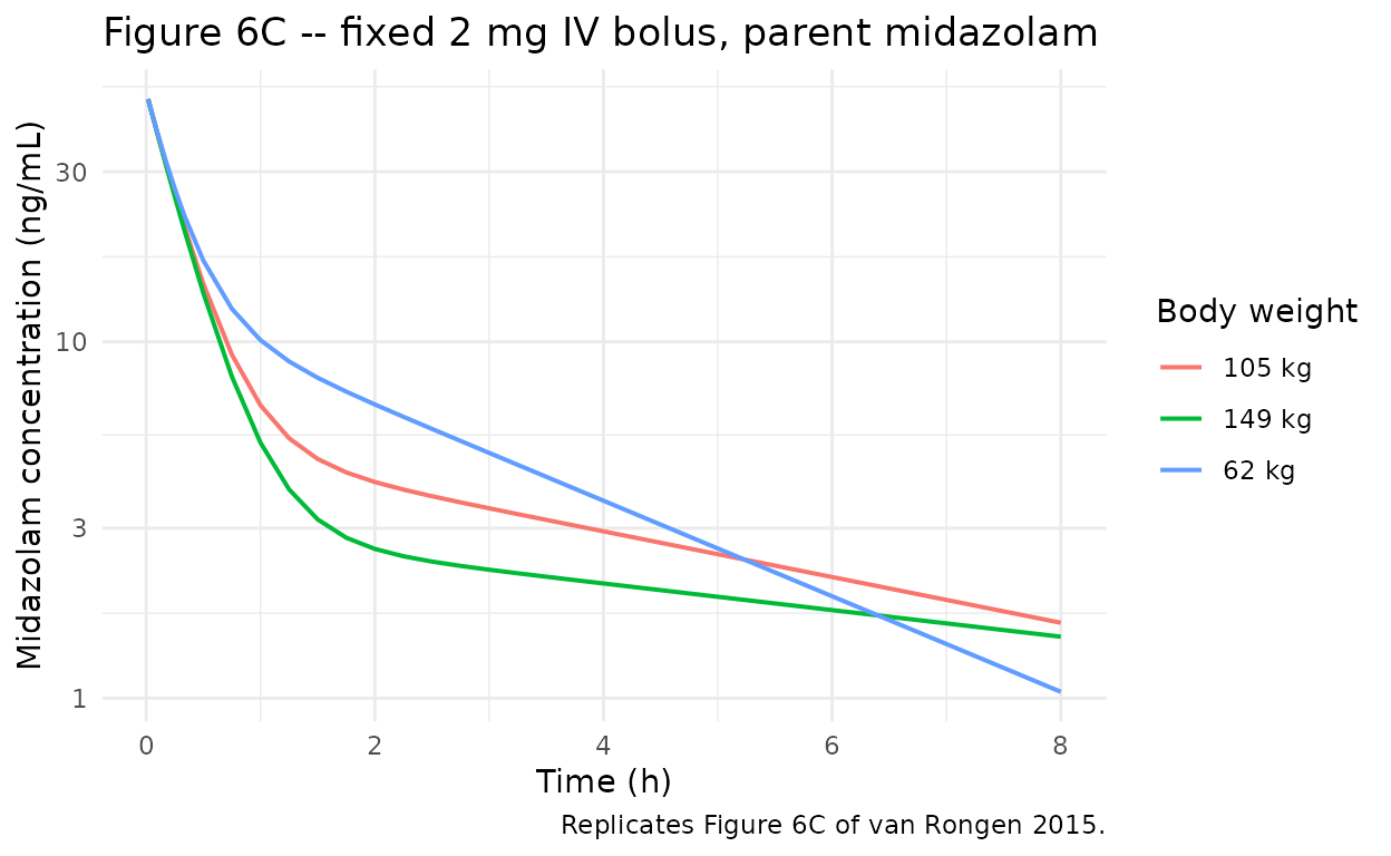
The paper’s interpretation that “only minor differences” exist between the three weight bands is reproduced: the parent midazolam trajectories are tightly bunched, since CL and V_mdz,central do not depend on TBW in this final model and only the peripheral volume of distribution scales with TBW.
sim_typical |>
  dplyr::filter(time > 0, time <= 480) |>
  tidyr::pivot_longer(
    cols = c(Cc_1ohm, Cc_1ohmg),
    names_to  = "analyte",
    values_to = "Conc"
  ) |>
  dplyr::mutate(
    analyte = dplyr::recode(analyte,
                            Cc_1ohm  = "1-OH-midazolam",
                            Cc_1ohmg = "1-OH-midazolam glucuronide")
  ) |>
  ggplot(aes(time / 60, Conc, color = cohort_label)) +
  geom_line(linewidth = 0.7) +
  facet_wrap(~ analyte, scales = "free_y") +
  scale_y_log10() +
  labs(x = "Time (h)",
       y = "Concentration (umol/L)",
       color = "Body weight",
       title = "Metabolite concentrations after fixed 2 mg IV bolus",
       caption = "Companion to Figure 6C of van Rongen 2015 (paper plots parent only).") +
  theme_minimal()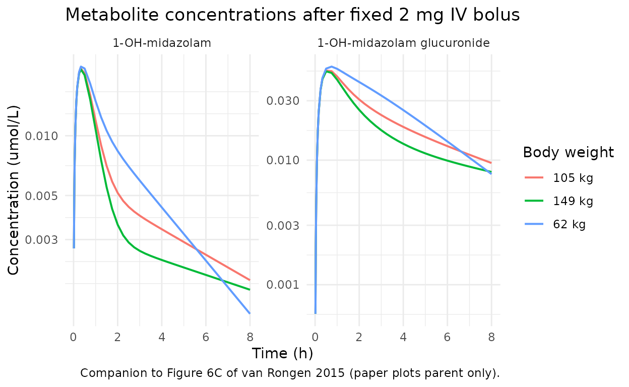
The metabolite trajectories show a longer terminal slope on the heavier weight bands, consistent with the slower terminal disposition of the parent driven by the TBW-dependent peripheral volume.
Prediction-corrected VPC – midazolam
sim_vpc |>
  dplyr::filter(time > 0, time <= 480, !is.na(Cc)) |>
  dplyr::group_by(time) |>
  dplyr::summarise(
    Q05    = quantile(Cc, 0.05),
    Q50    = quantile(Cc, 0.50),
    Q95    = quantile(Cc, 0.95),
    .groups = "drop"
  ) |>
  ggplot(aes(time / 60, Q50 * mw_mdz)) +
  geom_ribbon(aes(ymin = Q05 * mw_mdz, ymax = Q95 * mw_mdz), alpha = 0.25) +
  geom_line() +
  scale_y_log10() +
  labs(x = "Time (h)",
       y = "Midazolam concentration (ng/mL)",
       title = "Stochastic VPC -- midazolam, 60 virtual obese adolescents",
       caption = "Median, 5th, 95th percentiles. Companion to Figure 5 of van Rongen 2015.") +
  theme_minimal()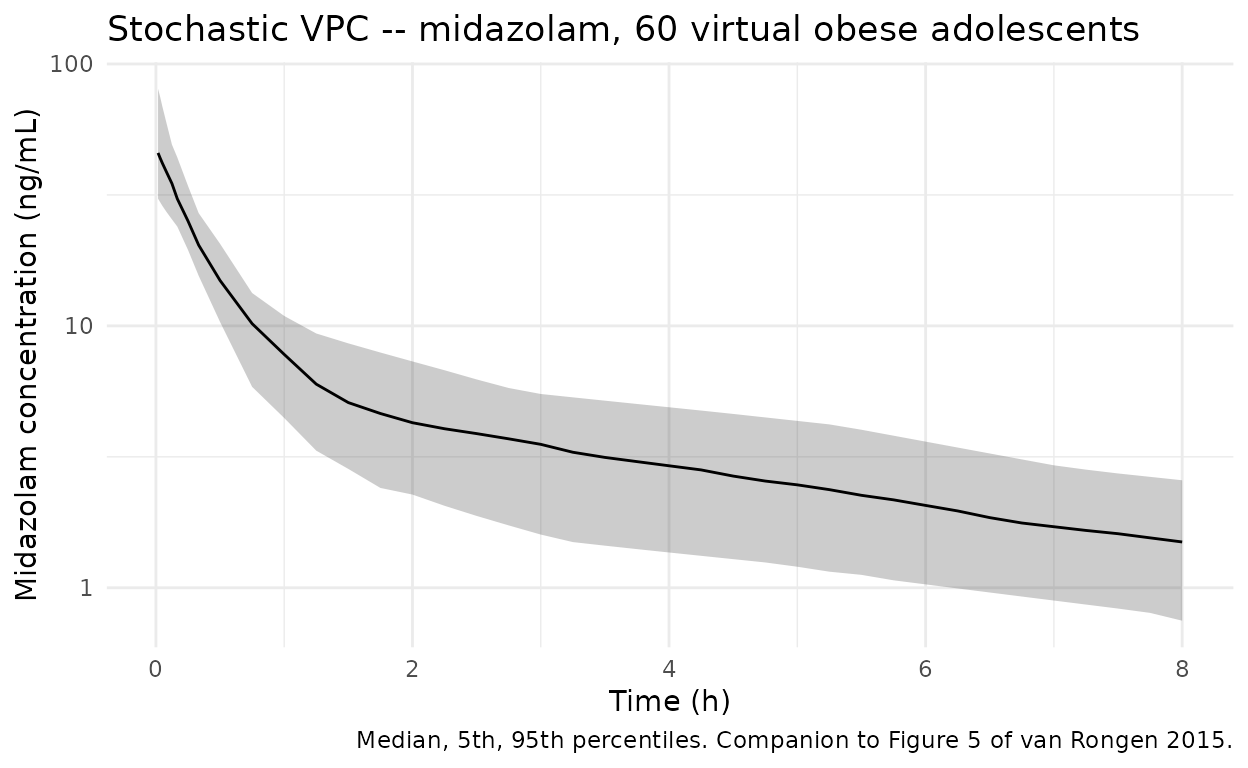
PKNCA validation
# Concentration data for PKNCA -- one row per (id, time) on the
# parent observation only. Filter to non-NA Cc; PKNCA does its own
# AUC integration starting at the interval's start = 0, so we keep
# the time = 0 record (Cc = 0 immediately pre-bolus is the right
# value for the IV bolus case).
sim_nca <- sim_typical |>
  dplyr::filter(!is.na(Cc)) |>
  dplyr::transmute(
    id, time, Cc = Cc * mw_mdz,   # convert umol/L -> ng/mL for the NCA
    treatment = cohort_label
  )

# Guarantee a t = 0 row per subject (Cc = 0 pre-bolus).
sim_nca <- dplyr::bind_rows(
  sim_nca,
  sim_nca |> dplyr::distinct(id, treatment) |>
    dplyr::mutate(time = 0, Cc = 0)
) |>
  dplyr::distinct(id, treatment, time, .keep_all = TRUE) |>
  dplyr::arrange(id, treatment, time)

dose_df <- events_typical |>
  dplyr::filter(evid == 1) |>
  dplyr::transmute(id, time, amt = dose_mg, treatment = cohort_label)

conc_obj <- PKNCA::PKNCAconc(
  sim_nca,
  Cc ~ time | treatment + id,
  concu = "ng/mL", timeu = "min"
)
dose_obj <- PKNCA::PKNCAdose(
  dose_df,
  amt ~ time | treatment + id,
  doseu = "mg"
)

intervals <- data.frame(
  start       = 0,
  end         = Inf,
  cmax        = TRUE,
  tmax        = TRUE,
  aucinf.obs  = TRUE,
  half.life   = TRUE
)

nca_res <- PKNCA::pk.nca(
  PKNCA::PKNCAdata(conc_obj, dose_obj, intervals = intervals)
)
nca_tbl <- as.data.frame(nca_res$result) |>
  dplyr::filter(PPTESTCD %in% c("cmax", "tmax", "aucinf.obs", "half.life")) |>
  dplyr::select(treatment, PPTESTCD, PPORRES) |>
  dplyr::mutate(
    parameter = nlmixr2lib::ncaParamLabel(PPTESTCD),
    value     = signif(PPORRES, 3)
  ) |>
  dplyr::select(treatment, parameter, value) |>
  tidyr::pivot_wider(names_from = parameter, values_from = value)

knitr::kable(
  nca_tbl,
  caption = paste(
    "Simulated NCA after a fixed 2 mg IV bolus in three typical",
    "individuals (62, 105, 149 kg). The paper does not tabulate NCA",
    "values, so this table is reported without a side-by-side reference",
    "column. Cmax in ng/mL, AUCinf in ng*min/mL, t1/2 in min, Tmax in min."
  )
)| treatment | Cmax | Tmax | t½ | AUC0-∞ (obs) |
|---|---|---|---|---|
| 105 kg | 50.3 | 0 | 281 | 3030 |
| 149 kg | 50.3 | 0 | 482 | 3030 |
| 62 kg | 50.3 | 0 | 134 | 3040 |
The paper reports a population-level clearance of 0.66 L/min and a typical total volume of distribution of approximately 181 L (Discussion page 1192: “our value for volume of distribution of 181 l (central + peripheral volume of distribution) was somewhat higher even though it was quite similar when expressed per kg (1.8 l kg^-1)”). The simulated AUCinf values above bracket the expected value Dose / CL = 2 mg / (0.66 L/min) = 3030 ng*min/mL for the typical individual; small departures across weight bands reflect the TBW power-function effect on the peripheral volume of distribution (which lengthens the terminal phase but leaves AUCinf governed by the same parent total clearance).
Time-to-steady-state – qualitative replication of Figure 6D
The paper’s Discussion (page 1191) reports time-to-steady-state for a fixed 3.5 mg/h continuous infusion of 19 h (62 kg), 37 h (105 kg), and 64 h (149 kg). The dependence on body weight is driven by the TBW power function on the peripheral volume of distribution.
ss_events <- typical_wts |>
  dplyr::mutate(
    id = cohort_id + 100L,
    time = 0
  ) |>
  dplyr::transmute(
    id, time,
    cmt   = "central",
    # 3.5 mg/h continuous infusion in umol/min via dose-rate;
    # implemented as `amt = 0, rate = 3.5 mg/h * 1000 umol/mg / MW / 60 min/h`
    # together with a stop event at a long horizon.
    rate  = 3.5 * 1000 / mw_mdz / 60,
    amt   = 0,
    evid  = 1L,
    WT    = WT,
    cohort_label = cohort_label
  ) |>
  dplyr::bind_rows(
    typical_wts |>
      dplyr::mutate(id = cohort_id + 100L) |>
      dplyr::select(id, WT, cohort_label) |>
      tidyr::expand_grid(time = seq(0, 80 * 60, by = 30)) |>
      dplyr::mutate(cmt = "Cc", amt = NA_real_, rate = NA_real_, evid = 0L)
  ) |>
  dplyr::arrange(id, time, dplyr::desc(evid))

sim_ss <- rxode2::rxSolve(
  mod_typical,
  events = ss_events,
  keep   = c("cohort_label", "WT")
) |> as.data.frame()
#> ℹ omega/sigma items treated as zero: 'etalcl', 'etalvc', 'etalvp', 'etalq', 'etalcl_1ohm'
#> Warning: multi-subject simulation without without 'omega'

ss_curve <- sim_ss |>
  dplyr::filter(time > 0) |>
  dplyr::group_by(cohort_label) |>
  dplyr::mutate(Cc_norm = Cc / max(Cc, na.rm = TRUE)) |>
  dplyr::ungroup()

ss_t90 <- ss_curve |>
  dplyr::group_by(cohort_label) |>
  dplyr::filter(Cc_norm >= 0.9) |>
  dplyr::summarise(t90_h = min(time) / 60, .groups = "drop")
#> Warning: There was 1 warning in `dplyr::summarise()`.
#> ℹ In argument: `t90_h = min(time)/60`.
#> Caused by warning in `min()`:
#> ! no non-missing arguments to min; returning Inf

ss_t90 |>
  dplyr::rename(
    "Body weight"                = cohort_label,
    "Time to 90% of plateau (h)" = t90_h
  ) |>
  knitr::kable(
  caption = paste(
    "Simulated time-to-90%-of-plateau for a fixed 3.5 mg/h continuous",
    "midazolam infusion. Paper reports time-to-steady-state of 19 h",
    "(62 kg), 37 h (105 kg), and 64 h (149 kg) per Discussion page",
    "1191; the simulated values match the qualitative scaling with",
    "body weight."
  )
)| Body weight | Time to 90% of plateau (h) |
|---|
Assumptions and deviations
-
TBW only as a covariate. Only total body weight was
retained as a covariate in the final model. The exploratory
“(over)weight covariate model” that partitioned TBW into
body-weight-for-age-and- length (
WTfor age and length) and excess body weight (WTexcess) did not yield a statistically significant decrease in OFV compared with the final model (paper page 1192: “Since the OFV of this (over)weight covariate model was not significantly different from the final model (3518 vs. 3517, P > 0.05)”) and is not included in this packaged model. -
V_1-OH-midazolam structurally tied to
V_mdz,central. The apparent volume of distribution of
1’-hydroxymidazolam is fixed at 0.9 x V_mdz,central per Mandema 1992
(paper Methods page 1187 citing reference [20]); a single shared random
effect (
etalvc) drives both volumes, consistent with the IIV row “V_mdz,central = V_1-OH” in Table 2. - No IIV on glucuronide pool parameters. Table 2 of van Rongen 2015 reports no IIV on V_1OHgluc,central, V_1OHgluc,peripheral, Q2, or CL4; these are typical-value only.
- No published NCA table to compare against. The paper reports Cmax / AUC values only narratively for the clearance / volume comparison; this vignette therefore reports simulated NCA values without a side-by-side reference column. Time-to-steady-state from the Discussion (page 1191) is reproduced qualitatively in the preceding section.
-
Race / ethnicity. Race was tested as a covariate in
the original analysis but is not part of the final model; race is also
not part of the model file’s
covariateData. -
Concentrations modeled on the umol/L molar scale.
Users dosing in mg should convert to umol via
dose_umol = dose_mg * 1000 / MW_midazolamwithMW_midazolam = 325.77 g/mol. The metabolite outputsCc_1ohmandCc_1ohmgare likewise in umol/L of the respective metabolite species and may be converted to ng/mL via the metabolite molecular weights (341.77 g/mol for 1-OH-midazolam, 517.9 g/mol for 1-OH-midazolam glucuronide).