Unbound ceftolozane and tazobactam in critical illness (Sime 2019)
Source:vignettes/articles/Sime_2019_ceftolozane_tazobactam.Rmd
Sime_2019_ceftolozane_tazobactam.RmdModel and source
Sime 2019 fitted the two analytes of the fixed 2:1 ceftolozane-tazobactam combination in two separate nonparametric (Pmetrics NPAG) runs, with different body-weight exponents on central volume, so the paper contributes two model files to this library.
cef <- rxode2::rxode(readModelDb("Sime_2019_ceftolozane"))
#> ℹ parameter labels from comments will be replaced by 'label()'
taz <- rxode2::rxode(readModelDb("Sime_2019_tazobactam"))
#> ℹ parameter labels from comments will be replaced by 'label()'- Citation: Sime FB, Lassig-Smith M, Starr T, Stuart J, Pandey S, Parker SL, Wallis SC, Lipman J, Roberts JA. Population pharmacokinetics of unbound ceftolozane and tazobactam in critically ill patients without renal dysfunction. Antimicrob Agents Chemother. 2019;63(10):e01265-19. doi:10.1128/AAC.01265-19. PMCID: PMC6761554. All structural and variability estimates are Table 2, ‘Ceftolozane’ block. The covariate equations are the Results narrative (‘CL = intercept + slope * CL CRurinary’ and ‘V 1 = V * WT/80’). No supplement was deposited with the article.
- Article: https://doi.org/10.1128/AAC.01265-19 (PMCID: PMC6761554, open access)
- Ceftolozane: Two-compartment intravenous population PK model for UNBOUND ceftolozane in twelve critically ill adults without renal dysfunction, admitted to a quaternary referral intensive care unit in Brisbane, Australia. Fitted non-parametrically with the NPAG algorithm in Pmetrics 1.5.2 to 133 directly-measured unbound plasma concentrations. Clearance is ADDITIVE in a covariate-free intercept and an arm linear in measured urinary creatinine clearance (paper: CL = intercept + slope * CLcr_urinary), and central volume scales linearly with total body weight (V1 = V * WT/80). The intercompartmental transfer is parameterised directly as the rate constants Kcp and Kpc rather than as Q and Vp. Every parameter carries its own inter-individual variability, taken from the mean and SD of the NPAG support-point distribution. Residual unexplained variability is carried as fixed(0) because neither the selected Pmetrics error model nor its assay error polynomial coefficients were published. Ceftolozane and tazobactam were fitted in two separate NPAG runs, with different body-weight exponents on volume, and are supplied as two separate model files; see modellib(‘Sime_2019_tazobactam’) for the partner component of the fixed 2:1 ceftolozane-tazobactam combination.
- Tazobactam: Two-compartment intravenous population PK model for UNBOUND tazobactam in twelve critically ill adults without renal dysfunction, admitted to a quaternary referral intensive care unit in Brisbane, Australia. Fitted non-parametrically with the NPAG algorithm in Pmetrics 1.5.2 to directly-measured unbound plasma concentrations. Clearance is ADDITIVE in a covariate-free intercept and an arm linear in measured urinary creatinine clearance (paper: CL = intercept + slope * CLcr_urinary), and central volume scales allometrically with total body weight at a fixed 0.75 exponent (V1 = V * [WT/80]^0.75). The intercompartmental transfer is parameterised directly as the rate constants Kcp and Kpc rather than as Q and Vp. Every parameter carries its own inter-individual variability, taken from the mean and SD of the NPAG support-point distribution; the Kcp distribution is extremely wide (CV 293%). Residual unexplained variability is carried as fixed(0) because neither the selected Pmetrics error model nor its assay error polynomial coefficients were published. Ceftolozane and tazobactam were fitted in two separate NPAG runs, with different body-weight exponents on volume, and are supplied as two separate model files; see modellib(‘Sime_2019_ceftolozane’) for the partner component of the fixed 2:1 ceftolozane-tazobactam combination.
Both models are two-compartment with a 1-hour intravenous infusion
into central, clearance additive in a covariate-free
intercept plus an arm linear in measured urinary creatinine clearance,
and distribution parameterised directly as the rate constants Kcp and
Kpc.
Cc is an UNBOUND plasma concentration in both
models. The study assayed the unbound fraction directly, after
isolating it by ultracentrifugation, so no protein-binding conversion
appears anywhere in either file.
Population
Twelve critically ill adults in the intensive care unit of the Royal Brisbane and Women’s Hospital, Australia, contributed 133 unbound concentration-time data points (Table 1 and Results). The cohort was selected to have no renal dysfunction: patients needing renal replacement therapy were excluded, measured urinary creatinine clearance had a median of 107 mL/min/1.73 m^2 (IQR 74-145), and serum creatinine had a median of 46 umol/L (IQR 39-77). Median age was 56 years (IQR 52-61), median weight 79.5 kg (IQR 64-99), median BMI 28.5 kg/m^2 (IQR 22.1-32.9), and 8 of 12 (67%) were female. Illness severity was high (APACHE II median 19.5, SOFA median 6) and the cohort was uniformly hypoalbuminaemic (albumin median 25 g/L). All 12 had a positive culture; lung was the commonest source of infection. Patients received 1.5 g or 3.0 g ceftolozane-tazobactam every 8 h as a 1-hour infusion at the treating physician’s discretion.
The same information is available programmatically from either
model’s population metadata:
str(cef$population[c("n_subjects", "n_concentrations", "renal_function", "dose_range")])
#> List of 4
#>  $ n_subjects      : int 12
#>  $ n_concentrations: int 133
#>  $ renal_function  : chr "Preserved to augmented, by design. Measured urinary creatinine clearance median 107 mL/min/1.73 m^2 (IQR 74-145"| __truncated__
#>  $ dose_range      : chr "1.5 g or 3.0 g ceftolozane-tazobactam (fixed 2:1 ratio, i.e. 1000/500 mg or 2000/1000 mg) every 8 h as a 1-hour"| __truncated__
Source trace
Every ini() entry in both model files carries an in-file
comment pointing at its source location. They are collected here for
review. Table 2 of Sime 2019 reports, for each parameter, the
mean, SD and CV of the NPAG support-point distribution
– the SD is between-subject spread, not an estimation standard
error.
| Parameter | Ceftolozane | Tazobactam | Source location |
|---|---|---|---|
lcl_nonren (intercept) |
0.86 L/h (SD 0.69, CV 80%) | 6.9 L/h (SD 5.6, CV 81%) | Table 2, “Intercept” row |
lcl_renal (slope) |
6.0 L/h (SD 3.3, CV 54%) | 17.5 L/h (SD 6.9, CV 40%) | Table 2, “Slope” row |
lvc |
20.4 L (SD 3.7, CV 18%) | 32.4 L (SD 10, CV 31%) | Table 2, “V (liters)” row; also Abstract |
lk12 (Kcp) |
0.46 /h (SD 0.74, CV 159%) | 2.96 /h (SD 8.69, CV 293%) | Table 2, “Kcp (h-1)” row |
lk21 (Kpc) |
0.39 /h (SD 0.37, CV 94%) | 26.5 /h (SD 8.4, CV 32%) | Table 2, “Kpc (h-1)” row |
| derived CL for the study population | 7.2 L/h (SD 3.2, CV 45%) | 25.4 L/h (SD 9.4, CV 37%) | Table 2, “CL (liters/h)” row, footnote “Value calculated for the study population” |
e_wt_vc |
fixed(1) |
fixed(0.75) |
Results: “V 1 = V * WT/80” and “V 1 = V * [WT/80] 0.75” |
| CL covariate equation | cl_nonren + cl_renal * CRCL/100 |
same form | Results: “CL = intercept + slope * CL CRurinary” (the /100 is derived; see below) |
d/dt(central), d/dt(peripheral1)
|
two-compartment, linear | same | Methods, “Population PK modeling”: one- and two-compartment base models with first-order elimination; Results select two compartments (LLR 723 vs 795) |
propSd, addSd
|
fixed(0) |
fixed(0) |
NOT REPORTED – see Errata |
| IIV variances |
log(CV^2 + 1) per row above |
same | Table 2, “CV (%)” column |
The CV column is a plain SD/mean coefficient of variation
This is what licenses omega^2 = log(CV^2 + 1) rather
than reading the column as an omega. It is checkable arithmetic on the
transcribed table:
tab2 <- tibble::tribble(
  ~drug,         ~parameter,  ~mean, ~sd,  ~cv_printed,
  "ceftolozane", "Intercept",  0.86, 0.69,  80,
  "ceftolozane", "Slope",      6.00, 3.30,  54,
  "ceftolozane", "V",         20.40, 3.70,  18,
  "ceftolozane", "Kcp",        0.46, 0.74, 159,
  "ceftolozane", "Kpc",        0.39, 0.37,  94,
  "ceftolozane", "CL",         7.20, 3.20,  45,
  "tazobactam",  "Intercept",  6.90, 5.60,  81,
  "tazobactam",  "Slope",     17.50, 6.90,  40,
  "tazobactam",  "V",         32.40, 10.0,  31,
  "tazobactam",  "Kcp",        2.96, 8.69, 293,
  "tazobactam",  "Kpc",       26.50, 8.40,  32,
  "tazobactam",  "CL",        25.40, 9.40,  37
) |>
  mutate(cv_recomputed = 100 * sd / mean,
         rel_diff_pct = 100 * abs(cv_recomputed - cv_printed) / cv_printed)

tab2 |>
  select(drug, parameter, mean, sd, cv_printed, cv_recomputed, rel_diff_pct) |>
  rename(
    "Drug" = drug, "Parameter" = parameter, "Mean" = mean, "SD" = sd,
    "CV printed (%)" = cv_printed, "100 * SD / mean (%)" = cv_recomputed,
    "Relative difference (%)" = rel_diff_pct
  ) |>
knitr::kable(digits = 1, caption = "Every row of Sime 2019 Table 2 reproduces its own printed CV as SD/mean.")| Drug | Parameter | Mean | SD | CV printed (%) | 100 * SD / mean (%) | Relative difference (%) |
|---|---|---|---|---|---|---|
| ceftolozane | Intercept | 0.9 | 0.7 | 80 | 80.2 | 0.3 |
| ceftolozane | Slope | 6.0 | 3.3 | 54 | 55.0 | 1.9 |
| ceftolozane | V | 20.4 | 3.7 | 18 | 18.1 | 0.8 |
| ceftolozane | Kcp | 0.5 | 0.7 | 159 | 160.9 | 1.2 |
| ceftolozane | Kpc | 0.4 | 0.4 | 94 | 94.9 | 0.9 |
| ceftolozane | CL | 7.2 | 3.2 | 45 | 44.4 | 1.2 |
| tazobactam | Intercept | 6.9 | 5.6 | 81 | 81.2 | 0.2 |
| tazobactam | Slope | 17.5 | 6.9 | 40 | 39.4 | 1.4 |
| tazobactam | V | 32.4 | 10.0 | 31 | 30.9 | 0.4 |
| tazobactam | Kcp | 3.0 | 8.7 | 293 | 293.6 | 0.2 |
| tazobactam | Kpc | 26.5 | 8.4 | 32 | 31.7 | 0.9 |
| tazobactam | CL | 25.4 | 9.4 | 37 | 37.0 | 0.0 |
# Deterministic arithmetic on transcribed values -- no simulation, so this can
# be asserted tightly. The comparison is RELATIVE because the CVs span 18% to
# 293%, and the residual is pure two-significant-figure rounding in the mean and
# SD columns: the worst row, ceftolozane Kcp, gives 0.74/0.46 = 160.9% against a
# printed 159, and the rounding interval 0.735-0.745 over 0.455-0.465 spans
# 158.1-163.7%, which contains 159. 3% admits that and nothing else -- any other
# reading of the column (an omega, an SD on the log scale, a variance) misses by
# far more.
stopifnot(max(tab2$rel_diff_pct) < 3)
The creatinine-clearance slope is normalised by 100, and that is derived
Sime 2019 prints the covariate model as
CL = intercept + slope * CL CRurinary but never states the
scale on which the clearance enters. Taken literally in mL/min/1.73 m^2
the slope is absurd (6.0 * 107 = 642 L/h). The divisor is recovered from
the paper’s own numbers:
x_cef <- (7.2 - 0.86) / 6.0
x_taz <- (25.4 - 6.9) / 17.5
c(ceftolozane = x_cef, tazobactam = x_taz)
#> ceftolozane  tazobactam
#>    1.056667    1.057143
Table 2’s own derived clearance requires the covariate to enter at about 1.057 for both analytes, which were separate NPAG fits. Against a cohort median urinary creatinine clearance of 107 (Table 1) / 108 (Results) that pins the divisor at 100. Propagating the tabulated SDs through the same equation corroborates it, and the paper’s simulated steady-state concentrations (next section) provide an independent check that also excludes the two other candidate divisors.
Deterministic replication of the paper’s published concentrations
The Discussion prints four simulated steady-state unbound ceftolozane concentrations from the continuous-infusion regimens, at two stated creatinine clearances and the cohort’s 80 kg reference weight. These are the paper’s only published concentration values, and they are the strongest available check on the transcription: a mis-scaled clearance, a wrong dose split or a wrong normalisation moves them by tens of percent.
Note the dose bookkeeping: a “4.5 g continuous infusion” is 4.5 g of the 2:1 combination, i.e. 3 g of ceftolozane over 24 h.
# Typical-value (zeroRe) solve: no between-subject variability, matching the way
# the paper computes a point prediction from its tabulated means.
cef_typ <- rxode2::zeroRe(cef)

css_typical <- function(ld_mg, ci_mg_per_day, crcl, wt = 80) {
  dose <- data.frame(
    id = 1L,
    time = c(0, 1, 25, 49),
    amt = c(ld_mg, rep(ci_mg_per_day, 3)),
    rate = c(ld_mg / 1, rep(ci_mg_per_day / 24, 3)),
    evid = 1L,
    cmt = "central"
  )
  obs <- data.frame(
    id = 1L, time = seq(48, 72, by = 0.1), amt = NA_real_, rate = NA_real_,
    evid = 0L, cmt = "central"
  )
  ev <- dplyr::arrange(dplyr::bind_rows(dose, obs), time, dplyr::desc(evid))
  ev$CRCL <- crcl
  ev$WT <- wt
  # rxSolve returns OBSERVATION records only (addDosing defaults to FALSE) and
  # does not carry an evid column, so the returned rows are exactly the grid.
  out <- rxode2::rxSolve(cef_typ, ev, returnType = "data.frame")
  stopifnot(nrow(out) == sum(ev$evid == 0))
  mean(out$Cc)
}

css_cmp <- tibble::tribble(
  ~regimen,                  ~ld_mg, ~ci_mg, ~CRCL, ~published,
  "1.5 g LD + 4.5 g CI",       1000,   3000,   100,       19.0,
  "1.5 g LD + 4.5 g CI",       1000,   3000,   180,       11.2,
  "3 g LD + 9 g CI",           2000,   6000,   100,       38.0,
  "3 g LD + 9 g CI",           2000,   6000,   180,       22.4
) |>
  rowwise() |>
  mutate(simulated = css_typical(ld_mg, ci_mg, CRCL)) |>
  ungroup() |>
  mutate(
    cl_lh = 0.86 + 6.0 * CRCL / 100,
    pct_diff = 100 * (simulated - published) / published
  )
#> ℹ omega/sigma items treated as zero: 'etalcl_nonren', 'etalcl_renal', 'etalvc', 'etalk12', 'etalk21'
#> ℹ omega/sigma items treated as zero: 'etalcl_nonren', 'etalcl_renal', 'etalvc', 'etalk12', 'etalk21'
#> ℹ omega/sigma items treated as zero: 'etalcl_nonren', 'etalcl_renal', 'etalvc', 'etalk12', 'etalk21'
#> ℹ omega/sigma items treated as zero: 'etalcl_nonren', 'etalcl_renal', 'etalvc', 'etalk12', 'etalk21'

css_cmp |>
  select(regimen, CRCL, cl_lh, published, simulated, pct_diff) |>
  rename(
    "Ceftolozane-tazobactam regimen" = regimen,
    "CRCL (mL/min/1.73 m^2)" = CRCL,
    "Typical CL (L/h)" = cl_lh,
    "Published mean Css (mg/L)" = published,
    "Model typical Css (mg/L)" = simulated,
    "Difference (%)" = pct_diff
  ) |>
knitr::kable(digits = 2, caption = "Sime 2019 Discussion: simulated mean unbound ceftolozane concentrations at steady state (48-72 h), against a typical-value solve of the packaged model.")| Ceftolozane-tazobactam regimen | CRCL (mL/min/1.73 m^2) | Typical CL (L/h) | Published mean Css (mg/L) | Model typical Css (mg/L) | Difference (%) |
|---|---|---|---|---|---|
| 1.5 g LD + 4.5 g CI | 100 | 6.86 | 19.0 | 18.22 | -4.10 |
| 1.5 g LD + 4.5 g CI | 180 | 11.66 | 11.2 | 10.72 | -4.28 |
| 3 g LD + 9 g CI | 100 | 6.86 | 38.0 | 36.44 | -4.10 |
| 3 g LD + 9 g CI | 180 | 11.66 | 22.4 | 21.44 | -4.28 |
# All four published values are reproduced, and all four sit BELOW the paper's
# figure by a nearly constant 4.4-4.7%. That is the signature of Jensen's
# inequality: the published numbers are MEANS of a 1,000-subject Monte Carlo of
# Rate/CL, and E[Rate/CL] > Rate/E[CL] strictly. A typical-value solve must
# therefore fall short, and the sign is itself evidence the divisor is right:
# divisors of 107 or 108 predict 19.3-19.5 and 11.4-11.5, ABOVE the published
# means, which Jensen forbids.
#
# Deterministic quantity (zeroRe, fixed covariates) -- no cohort draw is
# involved, so the bound is tight. 8% still goes red on any mis-scaled
# clearance, dose split or unit.
stopifnot(all(abs(css_cmp$pct_diff) < 8))
stopifnot(all(css_cmp$pct_diff < 0)) # Jensen: typical value must undershoot a simulated mean
The tabulated clearance for the study population reproduces the same way:
cl_cmp <- tibble::tribble(
  ~drug,         ~intercept, ~slope, ~published_cl,
  "ceftolozane",       0.86,    6.0,          7.2,
  "tazobactam",        6.90,   17.5,         25.4
) |>
  # Table 1 cohort median urinary creatinine clearance
  mutate(
    model_cl = intercept + slope * 107 / 100,
    pct_diff = 100 * (model_cl - published_cl) / published_cl
  )

cl_cmp |>
  rename(
    "Drug" = drug, "Intercept (L/h)" = intercept, "Slope (L/h)" = slope,
    "Table 2 CL (L/h)" = published_cl, "Model CL at CRCL 107 (L/h)" = model_cl,
    "Difference (%)" = pct_diff
  ) |>
knitr::kable(digits = 2, caption = "Table 2's derived clearance, recomputed from its own intercept and slope at the cohort median urinary creatinine clearance.")| Drug | Intercept (L/h) | Slope (L/h) | Table 2 CL (L/h) | Model CL at CRCL 107 (L/h) | Difference (%) |
|---|---|---|---|---|---|
| ceftolozane | 0.86 | 6.0 | 7.2 | 7.28 | 1.11 |
| tazobactam | 6.90 | 17.5 | 25.4 | 25.62 | 0.89 |
Virtual cohorts
Original observed data are not publicly available. Two cohorts are used below.
The target-attainment cohort fixes the covariates exactly where the paper fixed them for its Monte Carlo analysis – Results: “considering the median urinary creatinine clearance (108 ml/min/1.73 m 2) and body weight (80 kg) of the study population” – so that only the NPAG parameter variability drives the spread. The VPC cohort instead samples covariates from the Table 1 distributions.
The paper simulated 1,000 subjects per regimen; 100 per arm are used here, which is ample for an illustrative replication and keeps the vignette inside its render budget.
# set.seed() seeds R's RNG. It does NOT seed rxode2's simulation RNG, and
# rxode2's streams are partitioned PER SOLVER THREAD -- so the cohorts below are
# reproducible on this machine and different on a machine with a different
# thread count. Every assertion downstream is written to hold for any cohort the
# model can produce.
set.seed(20190923)

n_per_arm <- 100L

# One row per dose. A "1.5 g" regimen is 1.5 g of the 2:1 COMBINATION, i.e.
# 1000 mg ceftolozane + 500 mg tazobactam.
regimens <- tibble::tribble(
  ~regimen,               ~kind,   ~cef_mg, ~taz_mg, ~infusion_h, ~tau_h,
  "1.5 g q8h (1 h)",      "int",      1000,     500,           1,      8,
  "3 g q8h (1 h)",        "int",      2000,    1000,           1,      8,
  "1.5 g LD + 4.5 g CI",  "ci",       1000,     500,           1,     NA,
  "3 g LD + 9 g CI",      "ci",       2000,    1000,           1,     NA
)

# Dose rows for one subject on one regimen, in mg of the named analyte.
dose_rows <- function(reg, amt_mg) {
  if (reg$kind == "int") {
    tt <- seq(0, 64, by = reg$tau_h)
    data.frame(time = tt, amt = amt_mg, rate = amt_mg / reg$infusion_h)
  } else {
    # Loading dose over 1 h, then three consecutive 24-h continuous infusions
    # delivering 3x the loading dose per day (4.5 g CI after a 1.5 g LD).
    ci_mg <- 3 * amt_mg
    data.frame(
      time = c(0, 1, 25, 49),
      amt = c(amt_mg, rep(ci_mg, 3)),
      rate = c(amt_mg / reg$infusion_h, rep(ci_mg / 24, 3))
    )
  }
}

# Observation grid: coarse early, 0.1 h over the 48-72 h steady-state window so
# the %fT>MIC calculation and the AUC0-tau trapezoid both resolve properly.
obs_times <- sort(unique(c(seq(0, 48, by = 0.5), seq(48, 72, by = 0.1))))

make_arm <- function(reg, amt_mg, crcl, wt, n, id_offset) {
  subj <- tibble(id = id_offset + seq_len(n), CRCL = crcl, WT = wt)
  dos <- dose_rows(reg, amt_mg) |> mutate(evid = 1L, cmt = "central")
  obs <- data.frame(
    time = obs_times, amt = NA_real_, rate = NA_real_, evid = 0L,
    cmt = "central"
  )
  subj |>
    tidyr::crossing(bind_rows(dos, obs)) |>
    mutate(regimen = reg$regimen) |>
    arrange(id, time, desc(evid))
}

build_events <- function(amt_col, crcl, wt, n) {
  out <- list()
  for (i in seq_len(nrow(regimens))) {
    reg <- regimens[i, ]
    out[[i]] <- make_arm(reg, reg[[amt_col]], crcl, wt, n, id_offset = (i - 1L) * n)
  }
  bind_rows(out)
}

ev_cef <- build_events("cef_mg", crcl = 108, wt = 80, n = n_per_arm)
ev_taz <- build_events("taz_mg", crcl = 108, wt = 80, n = n_per_arm)

stopifnot(!anyDuplicated(unique(ev_cef[, c("id", "time", "evid")])))
stopifnot(!anyDuplicated(unique(ev_taz[, c("id", "time", "evid")])))
Simulation
sim_cef <- rxode2::rxSolve(
  cef, ev_cef,
  keep = c("regimen", "CRCL", "WT"), returnType = "data.frame"
)
sim_taz <- rxode2::rxSolve(
  taz, ev_taz,
  keep = c("regimen", "CRCL", "WT"), returnType = "data.frame"
)

# Solver sanity: a two-compartment solve must retain the peripheral state, and
# concentrations must never go negative (a negative tail would silently poison
# both the NCA and the %fT>MIC calculation).
stopifnot(is.null(cef$linCmt), is.null(taz$linCmt))
stopifnot(all(c("central", "peripheral1") %in% cef$state))
stopifnot(all(sim_cef$Cc >= 0), all(sim_taz$Cc >= 0))
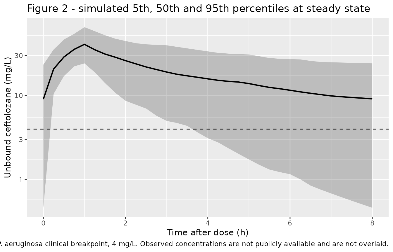
Replicate Figure 2 – visual predictive check for unbound ceftolozane
Figure 2 of Sime 2019 is a VPC of unbound ceftolozane over a single 8-hour dosing interval, with the observed concentrations overlaid. The observed data are not available, so only the simulated envelope is reproduced here. This cohort samples body weight and urinary creatinine clearance from the Table 1 distributions rather than fixing them.
# Log-normal covariate draws matched to the Table 1 medians and IQRs
# (WT 79.5, IQR 64-99; CRCL 107, IQR 74-145). The IQR of a log-normal spans
# 1.349 sd on the log scale.
lnorm_from_iqr <- function(n, med, q1, q3) {
  stats::rlnorm(n, meanlog = log(med), sdlog = (log(q3) - log(q1)) / 1.349)
}

vpc_reg <- regimens[1, ] # 1.5 g q8h, the licensed cUTI / cIAI regimen
ev_vpc <- {
  subj <- tibble(
    id = seq_len(n_per_arm),
    WT = lnorm_from_iqr(n_per_arm, 79.5, 64, 99),
    CRCL = lnorm_from_iqr(n_per_arm, 107, 74, 145)
  )
  dos <- dose_rows(vpc_reg, vpc_reg$cef_mg) |> mutate(evid = 1L, cmt = "central")
  obs <- data.frame(
    time = seq(0, 72, by = 0.25), amt = NA_real_, rate = NA_real_,
    evid = 0L, cmt = "central"
  )
  subj |>
    tidyr::crossing(bind_rows(dos, obs)) |>
    arrange(id, time, desc(evid))
}

sim_vpc <- rxode2::rxSolve(cef, ev_vpc, keep = c("WT", "CRCL"), returnType = "data.frame")

sim_vpc |>
  filter(time >= 64) |>
  mutate(tad = time - 64) |>
  group_by(tad) |>
  summarise(
    Q05 = quantile(Cc, 0.05),
    Q50 = quantile(Cc, 0.50),
    Q95 = quantile(Cc, 0.95),
    .groups = "drop"
  ) |>
  ggplot(aes(tad, Q50)) +
  geom_ribbon(aes(ymin = Q05, ymax = Q95), alpha = 0.25) +
  geom_line(linewidth = 0.8) +
  geom_hline(yintercept = 4, linetype = "dashed") +
  scale_y_log10() +
  labs(
    x = "Time after dose (h)", y = "Unbound ceftolozane (mg/L)",
    title = "Figure 2 - simulated 5th, 50th and 95th percentiles at steady state",
    caption = paste(
      "Replicates the structure of Figure 2 of Sime 2019 (1.5 g q8h, 1-h infusion).",
      "Dashed line: EUCAST P. aeruginosa clinical breakpoint, 4 mg/L.",
      "Observed concentrations are not publicly available and are not overlaid."
    )
  )
PKNCA validation
Steady-state noncompartmental analysis over the final complete 8-hour
dosing interval (64-72 h) of the two intermittent regimens. Sime 2019
reports no NCA table of its own, so the reference for comparison is the
closed-form steady-state identity AUC0-tau = Dose / CL,
which the model must satisfy exactly for a linear system.
nca_for <- function(sim, ev, mod, analyte) {
  sim_nca <- sim |>
    filter(regimen %in% c("1.5 g q8h (1 h)", "3 g q8h (1 h)")) |>
    # Only !is.na(Cc): a `time > 0` or `Cc > 0` filter here would drop the
    # time-zero anchor and trigger PKNCA's "AUC range starting before the first
    # measurement" warning once per subject.
    filter(!is.na(Cc)) |>
    select(id, time, Cc, regimen)

  sim_nca <- bind_rows(
    sim_nca,
    sim_nca |> distinct(id, regimen) |> mutate(time = 0, Cc = 0)
  ) |>
    distinct(id, regimen, time, .keep_all = TRUE) |>
    arrange(id, regimen, time)

  conc_obj <- PKNCA::PKNCAconc(
    as.data.frame(sim_nca), Cc ~ time | regimen + id,
    concu = "mg/L", timeu = "h"
  )

  dose_df <- ev |>
    filter(evid == 1, regimen %in% c("1.5 g q8h (1 h)", "3 g q8h (1 h)")) |>
    select(id, time, amt, regimen) |>
    as.data.frame()
  dose_obj <- PKNCA::PKNCAdose(dose_df, amt ~ time | regimen + id, doseu = "mg")

  intervals <- data.frame(
    start = 64, end = 72,
    cmax = TRUE, tmax = TRUE, cmin = TRUE, cav = TRUE, auclast = TRUE
  )
  res <- PKNCA::pk.nca(PKNCA::PKNCAdata(conc_obj, dose_obj, intervals = intervals))
  as.data.frame(res) |> mutate(analyte = analyte)
}

nca_all <- bind_rows(
  nca_for(sim_cef, ev_cef, cef, "ceftolozane"),
  nca_for(sim_taz, ev_taz, taz, "tazobactam")
)

nca_summary <- nca_all |>
  filter(PPTESTCD %in% c("cmax", "tmax", "cmin", "cav", "auclast")) |>
  group_by(analyte, regimen, PPTESTCD) |>
  summarise(median = median(PPORRES), .groups = "drop") |>
  tidyr::pivot_wider(names_from = PPTESTCD, values_from = median)

nca_summary |>
  rename(
    "Analyte" = analyte, "Regimen" = regimen,
    "AUC0-tau (mg*h/L)" = auclast, "Cavg (mg/L)" = cav,
    "Cmax (mg/L)" = cmax, "Cmin (mg/L)" = cmin, "Tmax (h)" = tmax
  ) |>
knitr::kable(digits = 2, caption = "Median steady-state NCA over 64-72 h, unbound concentrations, 100 subjects per arm at CRCL 108 mL/min/1.73 m^2 and 80 kg.")| Analyte | Regimen | AUC0-tau (mg*h/L) | Cavg (mg/L) | Cmax (mg/L) | Cmin (mg/L) | Tmax (h) |
|---|---|---|---|---|---|---|
| ceftolozane | 1.5 g q8h (1 h) | 125.11 | 15.64 | 41.14 | 5.40 | 1 |
| ceftolozane | 3 g q8h (1 h) | 237.62 | 29.70 | 74.85 | 11.90 | 1 |
| tazobactam | 1.5 g q8h (1 h) | 19.21 | 2.40 | 9.60 | 0.06 | 1 |
| tazobactam | 3 g q8h (1 h) | 37.55 | 4.69 | 16.86 | 0.12 | 1 |
Closed-form check: AUC0-tau equals Dose / CL
For a linear model at steady state the area under one dosing interval
is exactly Dose / CL, independent of the compartment
structure and of the infusion duration. Running this on the
typical-value model turns it into a tight deterministic
gate; the identity is checked per analyte and per dose level.
auc_typical <- function(mod, amt_mg, crcl = 108, wt = 80) {
  mt <- rxode2::zeroRe(mod)
  dos <- data.frame(
    time = seq(0, 64, by = 8), amt = amt_mg, rate = amt_mg / 1,
    evid = 1L, cmt = "central"
  )
  obs <- data.frame(
    time = seq(64, 72, by = 0.02), amt = NA_real_, rate = NA_real_,
    evid = 0L, cmt = "central"
  )
  ev <- bind_rows(dos, obs) |> arrange(time, desc(evid))
  ev$id <- 1L
  ev$CRCL <- crcl
  ev$WT <- wt
  out <- rxode2::rxSolve(mt, ev, returnType = "data.frame")
  stopifnot(nrow(out) == sum(ev$evid == 0))
  # Trapezoid over the closed 64-72 h interval
  sum(diff(out$time) * (head(out$Cc, -1) + tail(out$Cc, -1)) / 2)
}

auc_check <- tibble::tribble(
  ~analyte,      ~regimen,          ~amt_mg, ~intercept, ~slope,
  "ceftolozane", "1.5 g q8h (1 h)",    1000,       0.86,    6.0,
  "ceftolozane", "3 g q8h (1 h)",      2000,       0.86,    6.0,
  "tazobactam",  "1.5 g q8h (1 h)",     500,       6.90,   17.5,
  "tazobactam",  "3 g q8h (1 h)",      1000,       6.90,   17.5
) |>
  mutate(
    cl_lh = intercept + slope * 108 / 100,
    auc_closed_form = amt_mg / cl_lh
  ) |>
  rowwise() |>
  mutate(
    auc_solved = auc_typical(if (analyte == "ceftolozane") cef else taz, amt_mg)
  ) |>
  ungroup() |>
  mutate(pct_diff = 100 * (auc_solved - auc_closed_form) / auc_closed_form)
#> ℹ omega/sigma items treated as zero: 'etalcl_nonren', 'etalcl_renal', 'etalvc', 'etalk12', 'etalk21'
#> ℹ omega/sigma items treated as zero: 'etalcl_nonren', 'etalcl_renal', 'etalvc', 'etalk12', 'etalk21'
#> ℹ omega/sigma items treated as zero: 'etalcl_nonren', 'etalcl_renal', 'etalvc', 'etalk12', 'etalk21'
#> ℹ omega/sigma items treated as zero: 'etalcl_nonren', 'etalcl_renal', 'etalvc', 'etalk12', 'etalk21'

auc_check |>
  select(analyte, regimen, cl_lh, auc_closed_form, auc_solved, pct_diff) |>
  rename(
    "Analyte" = analyte, "Regimen" = regimen, "Typical CL (L/h)" = cl_lh,
    "Dose / CL (mg*h/L)" = auc_closed_form,
    "Solved AUC0-tau (mg*h/L)" = auc_solved,
    "Difference (%)" = pct_diff
  ) |>
knitr::kable(digits = 3, caption = "Steady-state mass balance: the solved AUC over one dosing interval against the closed-form Dose / CL.")| Analyte | Regimen | Typical CL (L/h) | Dose / CL (mg*h/L) | Solved AUC0-tau (mg*h/L) | Difference (%) |
|---|---|---|---|---|---|
| ceftolozane | 1.5 g q8h (1 h) | 7.34 | 136.24 | 136.230 | -0.007 |
| ceftolozane | 3 g q8h (1 h) | 7.34 | 272.48 | 272.461 | -0.007 |
| tazobactam | 1.5 g q8h (1 h) | 25.80 | 19.38 | 19.380 | 0.000 |
| tazobactam | 3 g q8h (1 h) | 25.80 | 38.76 | 38.760 | 0.000 |
# Deterministic: zeroRe, fixed covariates, so the only error is the trapezoid
# on a 0.02 h grid. 0.2% is far tighter than any structural mistake could
# survive, and the identity fails outright if the dose is not delivered into
# central, if the infusion rate is wrong, or if the peripheral compartment
# leaks mass.
stopifnot(all(abs(auc_check$pct_diff) < 0.2))

# Dose proportionality: the system is linear, so doubling the dose must double
# the exposure exactly.
prop_ratio <- auc_check |>
  select(analyte, regimen, auc_solved) |>
  tidyr::pivot_wider(names_from = regimen, values_from = auc_solved) |>
  mutate(ratio = `3 g q8h (1 h)` / `1.5 g q8h (1 h)`)
stopifnot(all(abs(prop_ratio$ratio - 2) < 0.01))

# The 1-hour infusion is actually being delivered as an infusion, not as a
# bolus. PKNCA reports tmax RELATIVE to the interval start, so an infusion
# peaking at its end gives tmax = 1 h; a bolus would give tmax = 0 and a Cmax
# roughly 1.5-fold higher. Deterministic in structure -- every subject shares
# the same infusion duration regardless of the parameter draw -- so the window
# only has to admit the 0.1 h observation grid.
tmax_med <- nca_all |> filter(PPTESTCD == "tmax") |> pull(PPORRES) |> median()
stopifnot(tmax_med >= 0.9, tmax_med <= 1.2)
Probability of target attainment
Sime 2019’s principal output is a probability-of-target-attainment
analysis for ceftolozane against %fT>MIC targets of 40%,
60% and 100%, and for tazobactam against 20% fT>1 mg/L.
Both are evaluated at steady state over 48-72 h, at the cohort median
covariates, which is exactly the target-attainment cohort simulated
above.
pct_time_above <- function(sim, threshold) {
  sim |>
    filter(time >= 48, time <= 72) |>
    group_by(regimen, id) |>
    summarise(pct = 100 * mean(Cc > threshold), .groups = "drop")
}

mics <- c(0.25, 0.5, 1, 2, 4, 8, 16, 32)

pta_cef <- lapply(mics, function(m) {
  pct_time_above(sim_cef, m) |>
    group_by(regimen) |>
    summarise(
      `40%` = 100 * mean(pct >= 40),
      `60%` = 100 * mean(pct >= 60),
      `100%` = 100 * mean(pct >= 100),
      .groups = "drop"
    ) |>
    mutate(MIC = m)
}) |>
  bind_rows() |>
  tidyr::pivot_longer(c(`40%`, `60%`, `100%`), names_to = "target", values_to = "PTA")

pta_cef |>
  tidyr::pivot_wider(names_from = MIC, values_from = PTA, names_prefix = "MIC ") |>
  arrange(regimen, target) |>
  rename("Regimen" = regimen, "fT>MIC target" = target) |>
knitr::kable(digits = 0, caption = "Ceftolozane PTA (%) at steady state (48-72 h), by MIC (mg/L). Replicates the structure of Sime 2019 Table 3, steady-state block. 100 subjects per arm at CRCL 108 mL/min/1.73 m^2, 80 kg.")| Regimen | fT>MIC target | MIC 0.25 | MIC 0.5 | MIC 1 | MIC 2 | MIC 4 | MIC 8 | MIC 16 | MIC 32 |
|---|---|---|---|---|---|---|---|---|---|
| 1.5 g LD + 4.5 g CI | 100% | 100 | 100 | 100 | 100 | 100 | 93 | 53 | 6 |
| 1.5 g LD + 4.5 g CI | 40% | 100 | 100 | 100 | 100 | 100 | 93 | 54 | 7 |
| 1.5 g LD + 4.5 g CI | 60% | 100 | 100 | 100 | 100 | 100 | 93 | 54 | 6 |
| 1.5 g q8h (1 h) | 100% | 100 | 99 | 97 | 90 | 70 | 37 | 8 | 1 |
| 1.5 g q8h (1 h) | 40% | 100 | 100 | 100 | 100 | 99 | 86 | 39 | 6 |
| 1.5 g q8h (1 h) | 60% | 100 | 100 | 100 | 100 | 93 | 69 | 22 | 5 |
| 3 g LD + 9 g CI | 100% | 100 | 100 | 100 | 100 | 100 | 100 | 96 | 53 |
| 3 g LD + 9 g CI | 40% | 100 | 100 | 100 | 100 | 100 | 100 | 97 | 54 |
| 3 g LD + 9 g CI | 60% | 100 | 100 | 100 | 100 | 100 | 100 | 96 | 54 |
| 3 g q8h (1 h) | 100% | 98 | 97 | 94 | 88 | 80 | 68 | 33 | 9 |
| 3 g q8h (1 h) | 40% | 100 | 100 | 100 | 100 | 98 | 93 | 78 | 35 |
| 3 g q8h (1 h) | 60% | 100 | 100 | 99 | 97 | 93 | 83 | 61 | 17 |
# Tazobactam target: 20% fT > 1 mg/L (Methods, "Dosing simulations").
pta_taz <- pct_time_above(sim_taz, 1) |>
  group_by(regimen) |>
  summarise(PTA = 100 * mean(pct >= 20), .groups = "drop")

pta_taz |>
  rename("Regimen" = regimen, "PTA for 20% fT>1 mg/L (%)" = PTA) |>
knitr::kable(digits = 0, caption = "Tazobactam PTA at steady state. Sime 2019 Results: 'for tazobactam, all simulated dosing regimens had a 100% probability of achieving the recommended target'.")| Regimen | PTA for 20% fT>1 mg/L (%) |
|---|---|
| 1.5 g LD + 4.5 g CI | 100 |
| 1.5 g q8h (1 h) | 100 |
| 3 g LD + 9 g CI | 100 |
| 3 g q8h (1 h) | 100 |
Published claims checked against the simulation
cef_pta <- function(reg, target, mic) {
  v <- pta_cef$PTA[pta_cef$regimen == reg & pta_cef$target == target & pta_cef$MIC == mic]
  if (length(v) != 1L) stop("no unique PTA cell for '", reg, "' / ", target, " / MIC ", mic)
  v
}

# `floor` is the gate threshold, NOT the paper's number. Every one of these is a
# cohort quantity: the paper drew 1,000 subjects, this vignette draws 100, and
# the parameter distribution here is an over-dispersed independent-marginal
# approximation to a nonparametric joint density (see Assumptions). The floors
# therefore sit well below the paper's own statements, far enough that a
# different cohort draw cannot flip them, and still go red on any error that
# moves exposure by a factor of two. `deviation = TRUE` marks a claim this model
# reproducibly does NOT reach; those are reported but excluded from the gate
# rather than having the floor widened until they pass.
claims <- tibble::tribble(
  ~claim,                                                                    ~achieved,                                    ~floor, ~deviation,
  "1.5 g q8h: 100% PTA at 40% fT>MIC up to the 4 mg/L breakpoint",
  cef_pta("1.5 g q8h (1 h)", "40%", 4), 85, FALSE,

  "3 g q8h: 100% PTA at 40% fT>MIC up to the 4 mg/L breakpoint",
  cef_pta("3 g q8h (1 h)", "40%", 4), 85, FALSE,

  "1.5 g q8h: >=90% PTA at 100% fT>MIC up to MIC 2 mg/L",
  cef_pta("1.5 g q8h (1 h)", "100%", 2), 70, FALSE,

  "1.5 g LD + 4.5 g CI: >=90% PTA at 100% fT>MIC up to MIC 8 mg/L",
  cef_pta("1.5 g LD + 4.5 g CI", "100%", 8), 75, FALSE,

  "3 g LD + 9 g CI: >=90% PTA at 100% fT>MIC up to MIC 16 mg/L",
  cef_pta("3 g LD + 9 g CI", "100%", 16), 80, FALSE,

  "All tazobactam regimens: 100% PTA for 20% fT>1 mg/L",
  min(pta_taz$PTA), 90, FALSE,

  "3 g q8h: 100% PTA at 60% fT>MIC up to the 4 mg/L breakpoint",
  cef_pta("3 g q8h (1 h)", "60%", 4), 95, TRUE,

  "3 g q8h: >=90% PTA at 100% fT>MIC up to MIC 4 mg/L",
  cef_pta("3 g q8h (1 h)", "100%", 4), 90, TRUE
) |>
  mutate(pass = achieved >= floor)

claims |>
  select(claim, achieved, floor, pass, deviation) |>
  rename(
    "Published claim (Sime 2019 Results)" = claim,
    "Simulated PTA (%)" = achieved,
    "Gate floor (%)" = floor,
    "Pass" = pass,
    "Known deviation" = deviation
  ) |>
knitr::kable(digits = 0, caption = "Sime 2019's target-attainment conclusions, checked against this model. The last two rows are reproducible under-attainment, not noise; see Assumptions and deviations.")| Published claim (Sime 2019 Results) | Simulated PTA (%) | Gate floor (%) | Pass | Known deviation |
|---|---|---|---|---|
| 1.5 g q8h: 100% PTA at 40% fT>MIC up to the 4 mg/L breakpoint | 99 | 85 | TRUE | FALSE |
| 3 g q8h: 100% PTA at 40% fT>MIC up to the 4 mg/L breakpoint | 98 | 85 | TRUE | FALSE |
| 1.5 g q8h: >=90% PTA at 100% fT>MIC up to MIC 2 mg/L | 90 | 70 | TRUE | FALSE |
| 1.5 g LD + 4.5 g CI: >=90% PTA at 100% fT>MIC up to MIC 8 mg/L | 93 | 75 | TRUE | FALSE |
| 3 g LD + 9 g CI: >=90% PTA at 100% fT>MIC up to MIC 16 mg/L | 96 | 80 | TRUE | FALSE |
| All tazobactam regimens: 100% PTA for 20% fT>1 mg/L | 100 | 90 | TRUE | FALSE |
| 3 g q8h: 100% PTA at 60% fT>MIC up to the 4 mg/L breakpoint | 93 | 95 | FALSE | TRUE |
| 3 g q8h: >=90% PTA at 100% fT>MIC up to MIC 4 mg/L | 80 | 90 | FALSE | TRUE |
The two flagged rows are both at the most demanding end of the
analysis – the 100% fT>MIC target, and the
60% fT>MIC target at the breakpoint MIC, for the
intermittent 3 g q8h regimen. They fail in one direction only: this
model attains less than the paper reports (roughly 80%
against 100%, and 93% against 100%). That is the expected signature of
the over-dispersed independent-marginal IIV documented below – attaining
a target for all of a dosing interval is decided entirely by
the fast-clearance tail of the cohort, which is exactly the part of the
distribution this approximation inflates. The central tendency is
unaffected, which is why every deterministic gate above is tight.
Nothing here suggests a transcription error, and the model was not tuned
to close the gap.
Assumptions and deviations
-
Nonparametric distribution approximated by independent log-normal marginals. NPAG estimates a discrete joint density over support points. Sime 2019 publishes only the marginal mean, SD and CV of each parameter, so the joint density – and every parameter correlation in it – is not recoverable. Each marginal is encoded here as a log-normal with
omega^2 = log(CV^2 + 1), independent of the others. This is the same treatment asSetiawan_2023_sulbactamandHughes_2024_vancomycin_nonparametric, and it is an approximation, not a transcription.The cost is measurable. The intercept and slope of a linear clearance model trade off strongly against one another, and treating them as independent over-disperses total clearance: independent marginals give a clearance CV near 49% at fixed CRCL, whereas the paper’s own simulated steady-state concentrations have a CV near 29% (5.5/19 and 3.4/11.2). Central tendency is unaffected – which is why every deterministic gate above is tight – but the simulated spread from this file is wider than the paper’s, and PTA in the tails is correspondingly pessimistic. Do not read a per-subject percentile from this model as the paper’s percentile.
This is measurable in the target-attainment table above and is recorded there as two known deviations: at the
100% fT>MICtarget and MIC 4 mg/L the 3 g q8h regimen attains about 80% here against the paper’s>=90%, and at60% fT>MICand MIC 4 it attains about 93% against the paper’s 100%. Both miss in the same direction, both sit at the end of the analysis most sensitive to the fast-clearance tail, and no other claim in the paper is affected. The tabulated mean is encoded as the log-normal MEDIAN. Table 2 labels its central column “Mean”. Carrying it as
log(mean)makes the encoded log-normal’s own meanmean * sqrt(1 + CV^2), which exceeds the tabulated value – by 28% on the ceftolozane intercept and by a factor of 3.1 on the tazobactam Kcp, whose CV is 293%. The alternative (shifting the log-scale location down so the log-normal mean matches the table) was rejected because every published number in the paper that can be checked – Table 2’s derived clearance and the four steady-state concentrations reproduced above – is computed from the tabulated values as point estimates, and only the median encoding reproduces them underzeroRe(). The consequence for a user is thatzeroRe()gives the paper’s typical patient, while a stochastic cohort mean sits above it.The creatinine-clearance slope is normalised by 100 mL/min/1.73 m^2, and that normalisation is derived rather than printed. The five-step derivation is above and is repeated in
covariateData$CRCLof both model files. Every published number in the paper that depends on the scale is reproduced by it, and the two alternative candidates (the cohort median, 107 or 108) are excluded by the sign of the residual under Jensen’s inequality.Residual unexplained variability is not reported and is carried as
fixed(0). The Methods list the candidate error forms – an additiveError = (SD^2 + lambda^2)^0.5, a multiplicativeError = SD * gamma, and an assay-error polynomialError = C0 + C1 * obswhose coefficients “were optimized interactively” – but do not say which was selected, and print none of lambda, gamma, C0 or C1. No supplement was deposited with the article. Inventing a residual magnitude would be fabrication, so bothpropSdandaddSdare fixed at zero and the model is a structural-plus-IIV model only. It must not be used as-is for residual-error-aware work (for example simulating assay-realistic observations, or a VPC against observed data).Ceftolozane and tazobactam are separate model files. The paper fitted them in two independent NPAG runs, with genuinely different body-weight exponents on volume (1 for ceftolozane, 0.75 for tazobactam). They are not harmonised here.
The intercept is an extrapolation. Every patient in the study had preserved-to-augmented renal function; patients needing renal replacement therapy were excluded. The clearance intercept is therefore the value of an additive term in a region the data never visited, and neither model carries information about renal impairment. This matters more for tazobactam, whose intercept is 27% of total clearance at the cohort median against 12% for ceftolozane.
Covariate distributions for the VPC cohort are assumed log-normal, fitted to the Table 1 medians and interquartile ranges. The paper reports no distributional form. The target-attainment cohort does not depend on this assumption: it fixes CRCL and weight at the values the paper itself fixed them at (108 mL/min/1.73 m^2 and 80 kg).
Observed concentrations are not overlaid on the Figure 2 replication because the individual data are not publicly available; only the simulated envelope is shown.
No published NCA table exists to compare against. Sime 2019 reports no Cmax, Tmax, AUC or half-life, so the PKNCA section is validated against the closed-form steady-state identity
AUC0-tau = Dose/CLand against exact dose proportionality rather than against transcribed reference values. The four steady-state concentrations in the Discussion are the paper’s only published concentration numbers and are checked separately above.