Vincristine (Nijstad 2022)
Source:vignettes/articles/Nijstad_2022_vincristine.Rmd
Nijstad_2022_vincristine.RmdModel and source
- Citation: Nijstad AL, Chu WY, de Vos-Kerkhof E, Enters-Weijnen CF, van de Velde ME, Kaspers GJL, Barnett S, Veal GJ, Lalmohamed A, Zwaan CM, Huitema ADR. A Population Pharmacokinetic Modelling Approach to Unravel the Complex Pharmacokinetics of Vincristine in Children. Pharm Res. 2022;39(10):2487-2495. doi:10.1007/s11095-022-03364-1
- Description: Semi-mechanistic population PK model for intravenous vincristine in children, adolescents and young adults (Nijstad 2022; n = 206, 0.04-33.9 years, 1297 plasma concentrations). Two-compartment linear disposition (CL, Vc, Q, Vp; allometric on body weight, exponents fixed at 0.75 and 1, 70 kg reference) plus a third, saturable compartment for vincristine bound to beta-tubulin, filled from the central amount at kon x (1 - bound/Bmax) and emptied at koff. The binding capacity Bmax scales with (WT/70)^1 x (AGE/18)^-0.199, so younger children carry more binding capacity per kg. IIV on CL, Q, Vc, Vp, kon and koff; inter-occasion variability on Bmax (one occasion per dose); proportional residual error.
- Article: https://doi.org/10.1007/s11095-022-03364-1 (open access)
Nijstad et al. pooled vincristine plasma concentrations from two prospective paediatric cohorts (the Netherlands and the UK) and three historical cohorts, and described them with a two-compartment model extended by a third, saturable compartment that stands for vincristine bound to beta-tubulin. The binding equation (Methods Eq. 1, Supplementary Table S1) is written in amounts:
dA(bound)/dt = kon x A(Vc) x (1 - A(bound)/Bmax) - koff x A(bound)-
CL,Qscale with(WT/70)^0.75;Vc,Vpwith(WT/70)^1 Bmax = Bmax_pop x (WT/70)^1 x (AGE/18)^-0.199
Clearance does not depend on age beyond body weight; the age effect sits on the binding capacity, which is larger per kilogram in younger children. The authors read this as a reason that young children tolerate higher vincristine doses.
Population
Nijstad 2022 Table I describes 206 patients (median age 8.3 years, range 0.04-33.9; 25 younger than 1 year) with 1297 plasma samples over 253 dosing occasions (1-5 per patient). Median body weight was 27.1 kg (range 2.9-126.0) and 48% were female. Patients came from an unrestricted paediatric oncology cohort at the Princess Maxima Center (Down syndrome excluded), a UK Ewing sarcoma cohort up to 24 years of age (20 centres), and three historical paediatric cohorts (Lee et al., van de Velde et al., Barnett et al.). Vincristine was dosed per local protocol at 1-2 mg/m^2 capped at 2 mg with infant reductions (median 1.6 mg, 1.4 mg/m^2, 0.05 mg/kg), as an IV bolus (214 occasions) or a 15-113 min infusion (39 occasions).
The same information is available programmatically via
readModelDb("Nijstad_2022_vincristine")()$population.
Source trace
The per-parameter origin is recorded as an in-file comment next to
each ini() entry in
inst/modeldb/specificDrugs/Nijstad_2022_vincristine.R. The
table below collects them in one place.
| Equation / parameter | Value | Source location |
|---|---|---|
lcl (CL, 70 kg) |
log(30.6) L/h | Table II |
lq (Q, 70 kg) |
log(63.2) L/h | Table II |
lvc (Vc, 70 kg) |
log(5.39) L | Table II |
lvp (Vp, 70 kg) |
log(400) L | Table II |
lbmax (Bmax, 70 kg, 18 years) |
log(0.525) mg | Table II |
lkon (kon) |
fixed(log(1300)) 1/h | Table II; Results ‘Model Development’ |
lkoff (koff) |
log(11.5) 1/h | Table II |
e_age_bmax |
-0.199 | Table II ‘Age on Bmax’ |
etalcl |
47.7% -> 0.205003 | Table II ‘IIV CL’ |
etalq |
38.1% -> 0.135545 | Table II ‘IIV Q’ |
etalvc |
122.5% -> 0.916541 | Table II ‘IIV Vc’ |
etalvp |
57.1% -> 0.282198 | Table II ‘IIV Vp’ |
etalkon |
126.5% -> 0.955598 | Table II ‘IIV k on’ |
etalkoff |
24.1% -> 0.0564569 | Table II ‘IIV k off’ |
etaiov_bmax_1 … etaiov_bmax_5
|
59.1% -> 0.299572 | Table II ‘IOV Bmax’; one occasion per dose (Methods) |
propSd |
0.301 | Table II ‘Proportional residual error’ |
| Central, peripheral and bound ODEs | n/a | Supplementary Table S1; Methods Eq. 1; Figure 1 |
| Allometry 0.75 (CL, Q) and 1 (Vc, Vp, Bmax), 70 kg | n/a | Methods and Results ‘Covariate Analysis’ |
(AGE/18)^e_age_bmax on Bmax |
n/a | Results ‘Covariate Analysis’ |
Pi = Ppop x exp(eta_i) |
n/a | Methods Eq. 2 |
Typical-value checks
mod <- readModelDb("Nijstad_2022_vincristine")
mod_typ <- rxode2::zeroRe(mod)
#> ℹ parameter labels from comments will be replaced by 'label()'
#> Warning: some etas defaulted to non-mu referenced, possible parsing error: etaiov_bmax_1, etaiov_bmax_2, etaiov_bmax_3, etaiov_bmax_4, etaiov_bmax_5
#> as a work-around try putting the mu-referenced expression on a simple line
#> Warning: some etas defaulted to non-mu referenced, possible parsing error: etaiov_bmax_1, etaiov_bmax_2, etaiov_bmax_3, etaiov_bmax_4, etaiov_bmax_5
#> as a work-around try putting the mu-referenced expression on a simple line

# Individual parameters for a set of (WT, AGE) pairs; the parameter columns
# come back on every output row.
typ_params <- function(wt, age) {
  ev <- data.frame(
    id = seq_along(wt), time = 0, evid = 1, amt = 1,
    cmt = "central", WT = wt, AGE = age, OCC = 1
  )
  ev <- dplyr::bind_rows(ev, dplyr::mutate(ev, time = 1, evid = 0, amt = 0))
  out <- rxode2::rxSolve(mod_typ, events = ev, returnType = "data.frame")
  # rxSolve omits the id column when only one subject is solved.
  if (!"id" %in% names(out)) out$id <- 1L
  out |>
    dplyr::group_by(id) |>
    dplyr::slice(1) |>
    dplyr::ungroup() |>
    dplyr::select(id, cl, q, vc, vp, bmax, kon, koff)
}

p70 <- typ_params(70, 18)
#> ℹ omega/sigma items treated as zero: 'etalcl', 'etalq', 'etalvc', 'etalvp', 'etalkon', 'etalkoff', 'etaiov_bmax_1', 'etaiov_bmax_2', 'etaiov_bmax_3', 'etaiov_bmax_4', 'etaiov_bmax_5'
knitr::kable(p70, digits = 4,
caption = "Typical parameters at 70 kg and 18 years (Table II).")| id | cl | q | vc | vp | bmax | kon | koff |
|---|---|---|---|---|---|---|---|
| 1 | 30.6 | 63.2 | 5.39 | 400 | 0.525 | 1300 | 11.5 |
stopifnot(
  abs(p70$cl - 30.6) < 1e-9, abs(p70$q - 63.2) < 1e-9,
  abs(p70$vc - 5.39) < 1e-9, abs(p70$vp - 400) < 1e-9,
  abs(p70$bmax - 0.525) < 1e-9, abs(p70$kon - 1300) < 1e-9,
  abs(p70$koff - 11.5) < 1e-9
)
Figure 2: clearance and binding capacity in the first two years
Figure 2 plots the typical clearance (right axis) and the typical
Bmax (left axis) against age from birth to 104 weeks, for typical
WHO-chart weights. The paper does not print the weights it used. The two
curves are read off the figure by the maintainers (pixel coordinates of
the published image, about 0.002 mg on Bmax and 0.03 L/h on CL), the
body weight at each age is recovered from the clearance curve alone by
inverting CL = 30.6 x (WT/70)^0.75, and the model’s Bmax
for that weight and age is compared with the Bmax curve. This tests the
weight and age terms of Bmax, which the clearance curve does not
involve. The recovered weights (3.6 kg at 2 weeks, 8.9 kg at 1 year,
11.5 kg at 2 years) are close to the WHO median weights for girls.
fig2 <- tibble::tribble(
  ~weeks, ~cl_fig, ~bmax_fig,
       2,   3.31,   0.0919,
       4,   3.63,   0.0907,
       8,   4.22,   0.0968,
      13,   4.72,   0.1018,
      17,   5.06,   0.1062,
      26,   5.61,   0.1112,
      39,   6.12,   0.1157,
      52,   6.52,   0.1188,
      65,   6.89,   0.1222,
      78,   7.19,   0.1252,
      91,   7.57,   0.1299,
     104,   7.88,   0.1330
) |>
  dplyr::mutate(
    AGE = weeks * 7 / 365.25,
    WT = 70 * (cl_fig / 30.6)^(4 / 3)
  )
fp <- typ_params(fig2$WT, fig2$AGE)
#> ℹ omega/sigma items treated as zero: 'etalcl', 'etalq', 'etalvc', 'etalvp', 'etalkon', 'etalkoff', 'etaiov_bmax_1', 'etaiov_bmax_2', 'etaiov_bmax_3', 'etaiov_bmax_4', 'etaiov_bmax_5'
#> Warning: multi-subject simulation without without 'omega'
fig2 <- fig2 |>
  dplyr::mutate(
    cl_model = fp$cl,
    bmax_model = fp$bmax,
    bmax_pct_diff = 100 * (bmax_model / bmax_fig - 1)
  )
knitr::kable(
  dplyr::select(fig2, weeks, WT, bmax_fig, bmax_model, bmax_pct_diff) |>
    dplyr::rename(
      "Age (weeks)" = weeks, "Weight from CL curve (kg)" = WT,
      "Bmax, Figure 2 (mg)" = bmax_fig, "Bmax, model (mg)" = bmax_model,
      "Difference (%)" = bmax_pct_diff
    ),
  digits = c(0, 2, 4, 4, 2),
  caption = "Model Bmax at the weights implied by the Figure 2 clearance curve."
)| Age (weeks) | Weight from CL curve (kg) | Bmax, Figure 2 (mg) | Bmax, model (mg) | Difference (%) |
|---|---|---|---|---|
| 2 | 3.61 | 0.0919 | 0.0920 | 0.15 |
| 4 | 4.08 | 0.0907 | 0.0907 | -0.02 |
| 8 | 4.99 | 0.0968 | 0.0966 | -0.24 |
| 13 | 5.79 | 0.1018 | 0.1018 | -0.01 |
| 17 | 6.35 | 0.1062 | 0.1059 | -0.31 |
| 26 | 7.29 | 0.1112 | 0.1116 | 0.39 |
| 39 | 8.19 | 0.1157 | 0.1157 | -0.04 |
| 52 | 8.91 | 0.1188 | 0.1188 | 0.03 |
| 65 | 9.59 | 0.1222 | 0.1224 | 0.13 |
| 78 | 10.15 | 0.1252 | 0.1249 | -0.24 |
| 91 | 10.87 | 0.1299 | 0.1297 | -0.13 |
| 104 | 11.47 | 0.1330 | 0.1333 | 0.21 |
# Typical-value replication on both sides; the residual is digitisation error
# (one pixel is about 1.5% of Bmax here).
stopifnot(max(abs(fig2$bmax_pct_diff)) < 3)

age_grid <- tibble::tibble(weeks = seq(2, 104, by = 1)) |>
  dplyr::mutate(
    AGE = weeks * 7 / 365.25,
    WT = exp(approx(log(fig2$weeks), log(fig2$WT), log(weeks), rule = 2)$y)
  )
gp <- typ_params(age_grid$WT, age_grid$AGE)
#> ℹ omega/sigma items treated as zero: 'etalcl', 'etalq', 'etalvc', 'etalvp', 'etalkon', 'etalkoff', 'etaiov_bmax_1', 'etaiov_bmax_2', 'etaiov_bmax_3', 'etaiov_bmax_4', 'etaiov_bmax_5'
#> Warning: multi-subject simulation without without 'omega'
age_grid <- age_grid |> dplyr::mutate(cl = gp$cl, bmax = gp$bmax)

ggplot(age_grid, aes(weeks)) +
  geom_line(aes(y = cl / 10, colour = "Clearance (L/h, /10)")) +
  geom_line(aes(y = bmax, colour = "Bmax (mg)")) +
  geom_point(data = fig2, aes(y = cl_fig / 10, colour = "Clearance (L/h, /10)"), shape = 1) +
  geom_point(data = fig2, aes(y = bmax_fig, colour = "Bmax (mg)"), shape = 1) +
  scale_y_continuous(sec.axis = sec_axis(~ . * 10, name = "Clearance (L/h)")) +
  labs(x = "Age (weeks)", y = "Maximum binding capacity (mg)", colour = NULL,
       title = "Typical CL and Bmax from birth to 2 years",
       caption = "Replicates Figure 2 of Nijstad 2022 (points: values read off the figure).") +
  theme(legend.position = "bottom")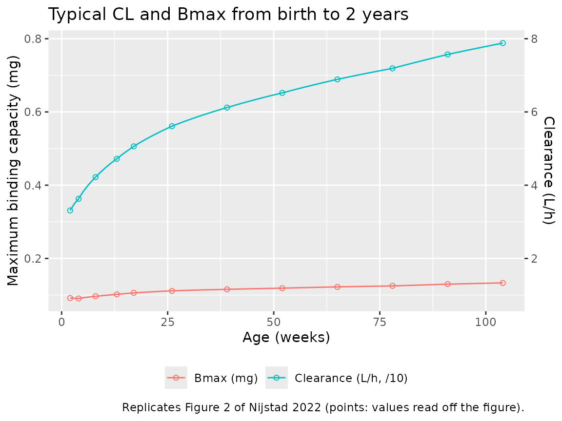
Virtual cohort
The observed data are not public. The virtual cohort follows the four
age strata of the paper’s prediction-corrected VPC (Supplementary Figure
S3): < 3.0, 3.0-8.9, 8.9-13.9
and > 13.9 years, 100 subjects each, with age drawn
uniformly within each stratum (> 13.9 capped at 25
years). Body weight comes from a log-linear interpolation of median
weight against age through the weights recovered from Figure 2 (2 weeks,
1 year and 2 years), the Table I cohort medians (8.3 years, 27.1 kg) and
70 kg at 18 years, with 15% log-normal scatter, truncated to the
observed 2.9-126.0 kg. Each subject gets one IV bolus of 1.5 mg/m^2
capped at 2 mg (the paper’s regimen A; Table I median 1.4 mg/m^2), with
BSA from the weight-only Costeff formula
BSA = (4 WT + 7) / (WT + 90), and is sampled for 72 hours
on occasion 1.
set.seed(20220819)
n_per <- 100
strata <- tibble::tibble(
  stratum = c("<3.0 years", "3.0-8.9 years", "8.9-13.9 years", ">13.9 years"),
  lo = c(0.04, 3.0, 8.9, 13.9),
  hi = c(3.0, 8.9, 13.9, 25)
)
wt_anchor <- tibble::tibble(
  age = c(2 * 7 / 365.25, 1, 2, 8.3, 18),
  wt = c(3.6, 8.9, 11.5, 27.1, 70)
)
median_wt <- function(age) {
  exp(approx(log(wt_anchor$age), log(wt_anchor$wt), log(age), rule = 2)$y)
}

subjects <- strata |>
  dplyr::slice(rep(seq_len(dplyr::n()), each = n_per)) |>
  dplyr::mutate(
    id = dplyr::row_number(),
    AGE = runif(dplyr::n(), lo, hi),
    WT = pmin(pmax(median_wt(AGE) * exp(rnorm(dplyr::n(), 0, 0.15)), 2.9), 126),
    BSA = (4 * WT + 7) / (WT + 90),
    dose = pmin(1.5 * BSA, 2)
  ) |>
  dplyr::select(id, stratum, AGE, WT, BSA, dose)

obs_times <- c(0, 0.05, 0.1, 0.25, 0.5, 0.75, 1, 1.5, 2, 3, 4, 6, 8, 12, 16,
               20, 24, 30, 36, 48, 60, 72)
events <- dplyr::bind_rows(
  dplyr::mutate(subjects, time = 0, evid = 1, amt = dose, cmt = "central"),
  tidyr::expand_grid(subjects, time = obs_times) |>
    dplyr::mutate(evid = 0, amt = 0, cmt = "central")
) |>
  dplyr::mutate(OCC = 1) |>
  dplyr::arrange(id, time, dplyr::desc(evid)) |>
  dplyr::select(id, time, evid, amt, cmt, WT, AGE, OCC, stratum, dose)

subjects |>
  dplyr::mutate(stratum = factor(stratum, levels = strata$stratum)) |>
  dplyr::group_by(stratum) |>
  dplyr::summarise(
    n = dplyr::n(), age_median = median(AGE), wt_median = median(WT),
    dose_median = median(dose), dose_per_kg = median(dose / WT),
    .groups = "drop"
  ) |>
  dplyr::rename(
    "Age stratum" = stratum, "Median age (years)" = age_median,
    "Median weight (kg)" = wt_median, "Median dose (mg)" = dose_median,
    "Median dose (mg/kg)" = dose_per_kg
  ) |>
knitr::kable(digits = 3, caption = "Virtual cohort by age stratum.")| Age stratum | n | Median age (years) | Median weight (kg) | Median dose (mg) | Median dose (mg/kg) |
|---|---|---|---|---|---|
| <3.0 years | 100 | 1.602 | 10.506 | 0.732 | 0.070 |
| 3.0-8.9 years | 100 | 5.812 | 22.474 | 1.292 | 0.057 |
| 8.9-13.9 years | 100 | 11.023 | 38.634 | 1.884 | 0.049 |
| >13.9 years | 100 | 18.697 | 64.350 | 2.000 | 0.031 |
Simulation
sim <- rxode2::rxSolve(
  mod, events = events,
  keep = c("stratum", "AGE", "WT"),
  returnType = "data.frame"
)
#> ℹ parameter labels from comments will be replaced by 'label()'
#> Warning: some etas defaulted to non-mu referenced, possible parsing error: etaiov_bmax_1, etaiov_bmax_2, etaiov_bmax_3, etaiov_bmax_4, etaiov_bmax_5
#> as a work-around try putting the mu-referenced expression on a simple line
stopifnot(!anyNA(sim$Cc))
sim$stratum <- factor(sim$stratum, levels = strata$stratum)
Supplementary Figure S3: VPC by age stratum
vpc <- sim |>
  dplyr::filter(time <= 27) |>
  dplyr::group_by(stratum, time) |>
  dplyr::summarise(
    Q05 = quantile(sim, 0.05), Q50 = median(sim), Q95 = quantile(sim, 0.95),
    .groups = "drop"
  )
ggplot(vpc, aes(time, Q50)) +
  geom_ribbon(aes(ymin = Q05, ymax = Q95), alpha = 0.25) +
  geom_line() +
  facet_wrap(~stratum, nrow = 1) +
  coord_cartesian(ylim = c(0, 30)) +
  labs(x = "Time after dose (hours)", y = "Plasma vincristine (ng/mL)",
       title = "Simulated median and 5th-95th percentiles, 1.5 mg/m^2 bolus",
       caption = "Compare with Supplementary Figure S3 of Nijstad 2022.")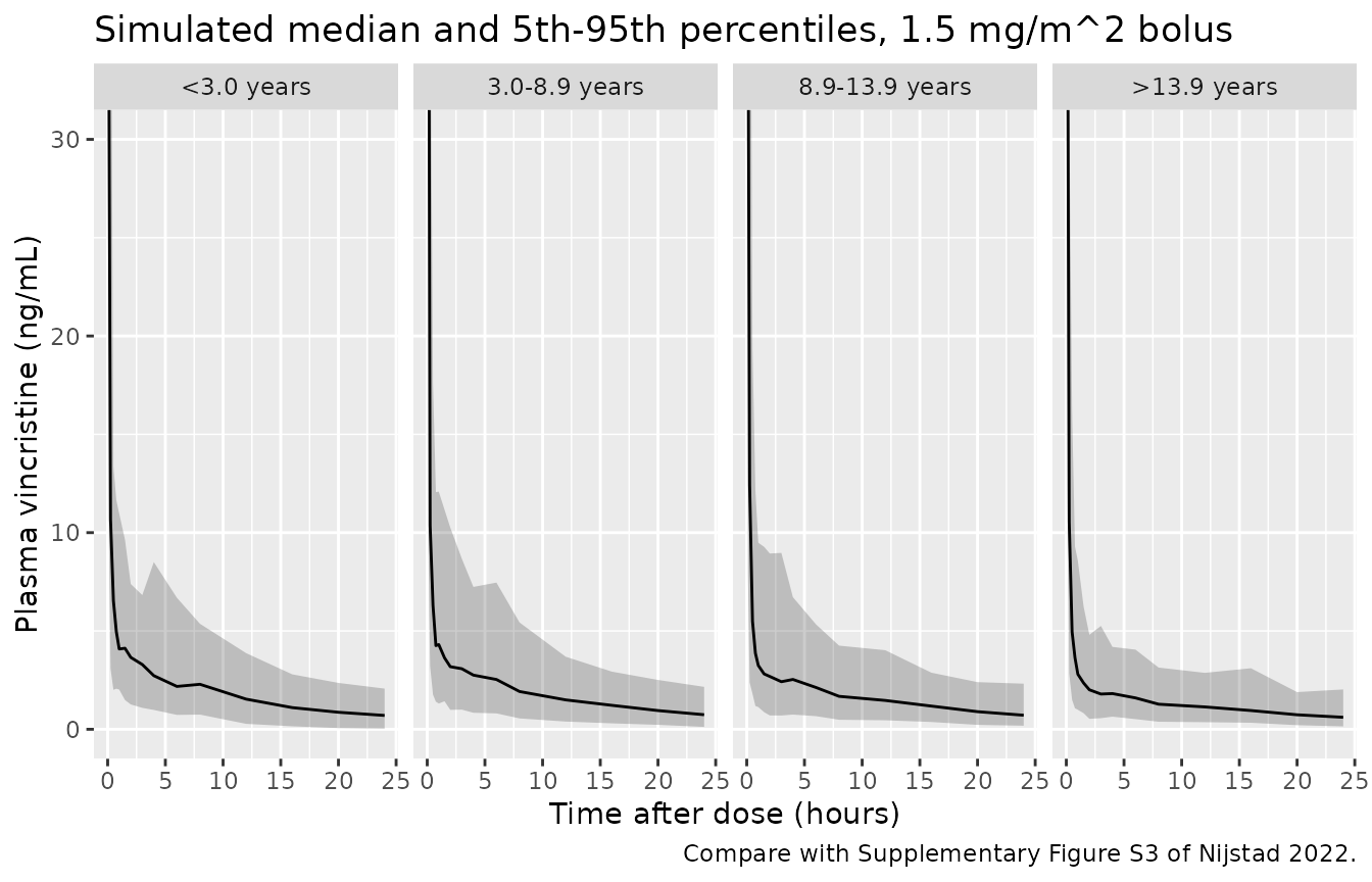
The observed medians of the published prediction-corrected VPC are read off Supplementary Figure S3 by the maintainers at 4, 8, 12 and 24 h. The simulated medians use an assumed dose rule rather than the trial doses, so the comparison is about the shape and level of the post-distribution profile, not an exact match.
s3_obs <- tibble::tribble(
  ~stratum,          ~time, ~obs_median,
  "<3.0 years",          4,  2.35,
  "<3.0 years",          8,  2.03,
  "<3.0 years",         12,  1.95,
  "<3.0 years",         24,  1.26,
  "3.0-8.9 years",       4,  1.86,
  "3.0-8.9 years",       8,  1.62,
  "3.0-8.9 years",      12,  1.54,
  "3.0-8.9 years",      24,  0.97,
  "8.9-13.9 years",      4,  2.35,
  "8.9-13.9 years",      8,  1.95,
  "8.9-13.9 years",     12,  1.54,
  "8.9-13.9 years",     24,  0.85,
  ">13.9 years",         4,  1.78,
  ">13.9 years",         8,  1.62,
  ">13.9 years",        12,  1.42,
  ">13.9 years",        24,  0.65
)
s3_cmp <- sim |>
  dplyr::filter(time %in% s3_obs$time) |>
  dplyr::group_by(stratum, time) |>
  dplyr::summarise(sim_median = median(sim), .groups = "drop") |>
  dplyr::mutate(stratum = as.character(stratum)) |>
  dplyr::inner_join(s3_obs, by = c("stratum", "time")) |>
  dplyr::mutate(ratio = sim_median / obs_median)
knitr::kable(
  s3_cmp |>
    dplyr::rename(
      "Age stratum" = stratum, "Time (h)" = time,
      "Simulated median (ng/mL)" = sim_median,
      "Observed median, Figure S3 (ng/mL)" = obs_median,
      "Simulated / observed" = ratio
    ),
  digits = 2,
  caption = "Simulated versus observed (Figure S3) median concentrations."
)| Age stratum | Time (h) | Simulated median (ng/mL) | Observed median, Figure S3 (ng/mL) | Simulated / observed |
|---|---|---|---|---|
| <3.0 years | 4 | 2.73 | 2.35 | 1.16 |
| <3.0 years | 8 | 2.29 | 2.03 | 1.13 |
| <3.0 years | 12 | 1.53 | 1.95 | 0.79 |
| <3.0 years | 24 | 0.70 | 1.26 | 0.56 |
| 3.0-8.9 years | 4 | 2.75 | 1.86 | 1.48 |
| 3.0-8.9 years | 8 | 1.92 | 1.62 | 1.19 |
| 3.0-8.9 years | 12 | 1.49 | 1.54 | 0.97 |
| 3.0-8.9 years | 24 | 0.74 | 0.97 | 0.76 |
| 8.9-13.9 years | 4 | 2.53 | 2.35 | 1.08 |
| 8.9-13.9 years | 8 | 1.68 | 1.95 | 0.86 |
| 8.9-13.9 years | 12 | 1.47 | 1.54 | 0.95 |
| 8.9-13.9 years | 24 | 0.71 | 0.85 | 0.84 |
| >13.9 years | 4 | 1.82 | 1.78 | 1.02 |
| >13.9 years | 8 | 1.28 | 1.62 | 0.79 |
| >13.9 years | 12 | 1.14 | 1.42 | 0.80 |
| >13.9 years | 24 | 0.61 | 0.65 | 0.94 |
stopifnot(
  nrow(s3_cmp) == nrow(s3_obs),
  # Centre: a mis-transcribed CL, volume, Bmax or unit moves every row.
  abs(log(median(s3_cmp$ratio))) < log(1.25),
  # Envelope: the dose rule and age mix are assumed, so allow a factor of 2.
  quantile(abs(log(s3_cmp$ratio)), 0.9) < log(2)
)
Across strata and times the simulated medians sit close to the observed ones. The largest gap is the youngest stratum at 24 h (simulated about half the observed median). That stratum is the most sensitive to the assumed dose rule and to how ages are spread between 2 weeks and 3 years, neither of which the paper reports per stratum.
PKNCA validation
The paper reports no NCA. PKNCA summarises the simulated single-dose
exposure by age stratum. The dose-normalised AUC falls with age mainly
because clearance grows with body weight; the larger per-kg binding
capacity of younger children pulls their concentrations down further at
low levels. Cmax here is the instantaneous concentration
right after the bolus (dose / Vc), which depends strongly on the very
variable Vc (IIV 122.5%); the earliest observed samples, taken minutes
after the dose, reach about 120 ng/mL (Supplementary Figure S1).
conc_df <- sim |>
  dplyr::filter(!is.na(Cc)) |>
  dplyr::mutate(Cc = pmax(Cc, 0), stratum = as.character(stratum)) |>
  dplyr::select(id, time, Cc, stratum)
dose_df <- events |>
  dplyr::filter(evid == 1) |>
  dplyr::select(id, time, amt, stratum)

nca <- PKNCA::pk.nca(PKNCA::PKNCAdata(
  PKNCA::PKNCAconc(conc_df, Cc ~ time | stratum + id),
  PKNCA::PKNCAdose(dose_df, amt ~ time | stratum + id),
  intervals = data.frame(
    start = 0, end = 72, cmax = TRUE, auclast = TRUE, half.life = TRUE
  )
))
nca_res <- as.data.frame(nca)
nca_tab <- nca_res |>
  dplyr::filter(PPTESTCD %in% c("cmax", "auclast", "half.life")) |>
  dplyr::left_join(dplyr::select(subjects, id, dose), by = "id") |>
  dplyr::mutate(
    PPORRES = ifelse(PPTESTCD == "auclast", PPORRES / dose, PPORRES),
    PPTESTCD = ifelse(PPTESTCD == "auclast", "auclast_per_mg", PPTESTCD)
  ) |>
  dplyr::group_by(stratum, PPTESTCD) |>
  dplyr::summarise(median = median(PPORRES, na.rm = TRUE), .groups = "drop") |>
  tidyr::pivot_wider(names_from = PPTESTCD, values_from = median) |>
  dplyr::mutate(stratum = factor(stratum, levels = strata$stratum)) |>
  dplyr::arrange(stratum)
knitr::kable(
  nca_tab |>
    dplyr::rename(
      "Age stratum" = stratum, "Cmax (ng/mL)" = cmax,
      "AUC0-72 per mg dose (ng*h/mL/mg)" = auclast_per_mg,
      "Terminal t1/2 (h)" = half.life
    ),
  digits = 2,
  caption = "Median simulated NCA by age stratum (1.5 mg/m^2 bolus, capped at 2 mg)."
)| Age stratum | AUC0-72 per mg dose (ng*h/mL/mg) | Cmax (ng/mL) | Terminal t1/2 (h) |
|---|---|---|---|
| <3.0 years | 139.71 | 1100.72 | 15.13 |
| 3.0-8.9 years | 78.45 | 880.10 | 18.52 |
| 8.9-13.9 years | 48.50 | 651.49 | 19.76 |
| >13.9 years | 33.24 | 344.32 | 22.29 |
Assumptions and deviations
-
IIV and IOV scale. Table II prints IIV and IOV as
percentages without saying how they were derived. They are read as CV%
and converted with
omega^2 = log(CV^2 + 1), the same reading used for the same group’s clofarabine model (Nijstad_2021_clofarabine). If they are instead100 x sqrt(omega^2), the variances of the two widest rows (Vc 122.5%, kon 126.5%) would be 1.50 and 1.60 rather than 0.92 and 0.96. - Rate constants are not scaled by weight. The paper applies allometric exponents to clearances (0.75) and volumes (1), and to Bmax (1); kon and koff carry no weight term. The Table II footnote says the non-Bmax population estimates “are adjusted to an individual value using allometric scaling”, which is read as applying to the clearances and volumes only.
-
Occasions. One occasion per dose, as in the paper;
up to five occasions per patient (Table I), so
OCCtakes values 1-5. Any other value gives the IIV-only Bmax. -
Units. Doses are in mg and volumes in L;
Ccis reported in ng/mL (1000 x central / vc) to match the paper’s figures and LLOQs. -
Age near zero. The age term
(AGE/18)^-0.199grows without bound as age approaches zero. The youngest patient in the cohort was about 2 weeks old (0.04 years); use the model below that age with caution. - Virtual cohort and doses. The weight-for-age curve, the uniform age draws within the Figure S3 strata, the Costeff BSA and the single 1.5 mg/m^2 (cap 2 mg) bolus are assumptions of this article, not the trial design; the trial dosed 1-2 mg/m^2 by local protocol with infant reductions, partly as 15-113 min infusions. The Figure S3 comparison is therefore descriptive.
-
Platelet count. Tested on Bmax and dropped
(unstable fits); recorded in
covariatesDataExcluded. - Below-LLOQ data. The paper included the first below-LLOQ sample at half the LLOQ; that is a data-handling choice and has no counterpart in the simulation model.