Brain delivery of plasma-protein-bound drugs (Pardridge 2023)

Model and source

• Citation: Pardridge WM (2023). Physiologically Based Pharmacokinetic Model of Brain Delivery of Plasma Protein Bound Drugs. Pharmaceutical Research 40(3):661-674. doi:10.1007/s11095-023-03484-2.
• Article: https://doi.org/10.1007/s11095-023-03484-2
• Supplement (Tables S1 and S2): https://doi.org/10.1007/s11095-023-03484-2 (Supplementary Information)

This paper contributes two models to nlmixr2lib, one per drug. Both share the same ODE structure and differ only in their drug-specific parameter values, exactly as the author built them (Table II has one column per drug):

pro <- readModelDb("Pardridge_2023_propranolol_pbpk")
imi <- readModelDb("Pardridge_2023_imipramine_pbpk")

pro_m <- rxode2::rxode2(pro)
imi_m <- rxode2::rxode2(imi)

What the model is for

Standard practice estimates the free (pharmacologically active) drug concentration in brain from the free fraction measured in vitro by equilibrium dialysis of plasma. Pardridge’s model asks whether that is valid when a drug is taken up by brain directly from its plasma-protein-bound pool - so-called plasma-protein-mediated uptake (PMU).

The mechanism is enhanced dissociation: within the brain capillary, contact with the endothelial glycocalyx raises the dissociation constant of the drug-protein complex above its in vitro value, so protein-bound drug becomes available to cross the blood-brain barrier during a single capillary transit without the protein itself leaving the circulation.

• Propranolol shows modest PMU, from the AGP-bound pool only (KG in vivo 19 uM vs KG in vitro 3.3 uM; albumin is unchanged).
• Imipramine shows strong PMU from both the AGP-bound and the albumin-bound pools (KG 90 vs 1.2 uM; KA >1,000 vs 42 uM).

Population

This is a deterministic simulation study, not a fit to individual data, so there is no study population in the popPK sense: there are no subjects, no inter-individual variability and no residual error. Every parameter is FIXED at a literature value or at a value the author calibrated by simulation.

The parameterisation represents a typical human: plasma albumin 800 uM and AGP 20 uM are human plasma concentrations (Table II, ref 12; the paper also simulates the metastatic-cancer values 600 uM and 70 uM), the in vitro dissociation constants are for human proteins, the total plasma concentration of 100 nM is a human pharmacologic level, and the oral propranolol pharmacokinetics are from human studies of an 80 mg dose in 70 kg subjects.

The species provenance is nonetheless mixed, and this is a genuine limitation rather than an approximation introduced here - see Assumptions and deviations below.

str(pro_m$meta$population)
#> List of 6
#>  $ species      : chr "human"
#>  $ n_subjects   : int NA
#>  $ n_studies    : int NA
#>  $ disease_state: chr "Not a fit to individual data. Deterministic simulation of a typical human parameterised from published human pl"| __truncated__
#>  $ dose_range   : chr "Non-steady-state model: single oral dose of 80 mg propranolol in a 70 kg subject, i.e. 4,600 nmol/kg, simulated"| __truncated__
#>  $ notes        : chr "Species provenance is mixed and should be understood before reuse. The plasma-protein concentrations (albumin 8"| __truncated__

Model structure

Eleven state variables (Table I). The arterial pool (LT0, GL0, GF0, LF0, AL0) is at instantaneous binding equilibrium and is computed algebraically; the brain capillary and brain pools are the seven ODE states.

Paper symbol	nlmixr2lib name	Meaning
LT0	Cc (output)	Total drug in arterial plasma
LF0	Cu_plasma_invitro (output)	Free drug in arterial plasma = C_u,plasma,in vitro
GL0, GF0, AL0	GL0, GF0, AL0 (algebraic, returned as columns)	AGP-bound drug, free AGP, and albumin-bound drug, arterial
LF	brain_vascular_drug_free	Free (bioavailable) drug in brain capillary = C_u,plasma,in vivo
GL	brain_vascular_drug_agp	AGP-bound drug in brain capillary
AL	brain_vascular_drug_alb	Albumin-bound drug in brain capillary
GF	brain_vascular_agp_free	Free (unbound) AGP in brain capillary
LM	brain_extravascular_drug_free	Free drug in brain = C_u,brain,in vivo
PL	brain_extravascular_drug_prot	Drug bound to brain cytoplasmic protein
PF	brain_extravascular_prot_free	Free brain cytoplasmic binding protein

The seven ODEs are Eqs 18-24 of the paper. The propranolol model additionally carries the paper’s one-compartment first-order oral model (Eq 13) as a depot / central pair so that LT0 can be driven by a dose event; the imipramine model has no dosing compartment because the paper states that “the non-steady state model was examined only for propranolol, as detailed pharmacokinetic (PK) parameters are not available following oral administration of imipramine”.

Source trace

Every ini() entry carries an in-file comment naming its source location. The table below collects them.

Paper symbol	Model parameter	Propranolol	Imipramine	Source
k1	lkoff_agp	1,140 /min	5,400 /min	Table II (refs 8, 9); k1 = k2 * KG,in vivo
k2	lkon_agp	0.06 /nM/min	0.06 /nM/min	Table II (ref 16)
k3	lkinflux_bbb	66 /min	150 /min	Table II (refs 8, 9); k3 = k10 * PS/F
k4	lkefflux_bbb	0.943 /min	2.1 /min	Table II (refs 8, 9); k4 = k3 * VP/VT
k5	lkon_brainprot	0.006 /nM/min	0.006 /nM/min	Table II; calibrated by simulation (Results)
k6	lkoff_brainprot	0.52 /min	0.5 /min	Table II (refs 17, 9)
k7	lkoff_alb	1,740 /min	6,000 /min	Table II (refs 8, 9); k7 = k8 * KA,in vivo
k8	lkon_alb	0.006 /nM/min	0.006 /nM/min	Table II (refs 18, 19)
k9	kmet_brain	0 /min	0 /min	Table II (refs 17, 20)
k10	lkflow_brain	60 /min	60 /min	Table II (ref 15)
KA in vitro	lkd_alb_invitro	290,000 nM	42,000 nM	Table II (refs 8, 13)
KG in vitro	lkd_agp_invitro	3,300 nM	1,200 nM	Table II (refs 8, 14)
AF	lc_alb	800,000 nM	800,000 nM	Table II (ref 12)
GT0	lc_agp	20,000 nM	20,000 nM	Table II (ref 12)
PT	lc_brainprot	5,000 nM	5,000 nM	Table II; calibrated (Results, Fig 2)
VP	lv_brain_vascular	0.01 L/kg	0.01 L/kg	Table II (ref 15)
VT	lv_brain_extravascular	0.7 L/kg	0.7 L/kg	Table II (ref 15)
LT0	c_plasma_ss	100 nM	100 nM	Table II (refs 10, 11)
b	lfdepot	0.3	n/a	Table II (ref 21)
s	dose (event table)	4,600 nmol/kg	n/a	Table II (ref 22); 80 mg in 70 kg
k	lka	0.023 /min	n/a	Table II (ref 22)
d	lkel	0.0027 /min	n/a	Table II (ref 22)
V	lvc	5.0 L/kg	n/a	Table II (ref 21)
Eqs 1-4 / 14-17	arterial algebra in model()	-	-	Methods
Eqs 18-24	the seven d/dt() lines	-	-	Methods
Eq 12	Kp,brain = (LM + PL)/LT0	-	-	Methods

Steady-state validation

The paper solved the steady state algebraically (Eqs 5-11, Mathematica Solve). The packaged models encode the differential form (Eqs 18-24), so the steady state is reached by integration. The two must agree.

solve_ss() overrides the parameters for one published simulation and integrates far past equilibrium.

# Zero-substitute: the log parameterisation cannot represent an exactly-zero
# protein concentration (Table S1 simulation 30 sets AF = GT0 = 0), so a
# numerically negligible 1e-9 nM stands in for a true zero.
ZERO <- 1e-9

solve_ss <- function(mod, p, tmax = 20000) {
  pars <- c(
    lkoff_agp       = log(p$k1),  lkon_agp        = log(p$k2),
    lkinflux_bbb    = log(p$k3),  lkefflux_bbb    = log(p$k4),
    lkon_brainprot  = log(p$k5),  lkoff_brainprot = log(p$k6),
    lkoff_alb       = log(p$k7),  lkon_alb        = log(p$k8),
    kmet_brain      = p$k9,       lkflow_brain    = log(p$k10),
    lkd_agp_invitro = log(p$KG),  lkd_alb_invitro = log(p$KA),
    lc_agp          = log(max(p$GT0, ZERO)),
    lc_alb          = log(max(p$AF,  ZERO)),
    lc_brainprot    = log(max(p$PT,  ZERO)),
    c_plasma_ss     = p$LT0
  )
  # The propranolol model additionally carries the oral PK parameters; they are
  # left at their defaults and contribute nothing when no dose is given.
  out <- rxode2::rxSolve(
    mod, rxode2::et(c(0, tmax)), params = pars,
    returnType = "data.frame", atol = 1e-12, rtol = 1e-12
  )
  x <- out[nrow(out), ]
  c(LF0 = x$Cu_plasma_invitro,
    GL  = x$brain_vascular_drug_agp,
    AL  = x$brain_vascular_drug_alb,
    LF  = x$Cu_plasma_invivo,
    GF  = x$brain_vascular_agp_free,
    LM  = x$Cu_brain,
    PL  = x$brain_extravascular_drug_prot,
    PF  = x$brain_extravascular_prot_free,
    Kp  = x$Cbrain_total / x$Cc)
}

Table III - propranolol steady-state simulations

basal_pro <- list(k1 = 1140, k2 = 0.06, k3 = 66, k4 = 0.943, k5 = 0.006,
                  k6 = 0.52, k7 = 1740, k8 = 0.006, k9 = 0, k10 = 60,
                  KG = 3300, KA = 290000, GT0 = 20000, AF = 800000,
                  PT = 5000, LT0 = 100)

tab3_changes <- list(
  "1 basal"                              = list(),
  "2 k1=198"                             = list(k1 = 198),
  "3 AF=600 uM; GT0=70 uM"               = list(AF = 600000, GT0 = 70000),
  "4 k1=11,400; k2=0.6"                  = list(k1 = 11400, k2 = 0.6),
  "5 k1=114; k2=0.006"                   = list(k1 = 114, k2 = 0.006),
  "6 k1=198; k3=66,600; k4=940"          = list(k1 = 198, k3 = 66000, k4 = 943),
  "7 k4=9.4"                             = list(k4 = 9.4),
  "8 k9=6"                               = list(k9 = 6),
  "9 k9=6; k10=6"                        = list(k9 = 6, k10 = 6),
  "10 k4=9.4; k9=6"                      = list(k4 = 9.4, k9 = 6)
)

tab3_sim <- lapply(tab3_changes, function(ch) {
  solve_ss(pro_m, modifyList(basal_pro, ch))
}) |> do.call(what = rbind) |> as.data.frame()

tab3_pub <- tibble::tribble(
  ~GL,   ~AL,   ~LF,   ~LM,   ~PL,  ~PF,   ~Kp,
  23.6,  55.8,  20.6,  20.6,  959,  4040,  9.8,
  61.7,  28.2,  10.2,  10.2,  526,  4473,  5.4,
  55.7,  29.6,  14.7,  14.7,  724,  4276,  7.4,
  22.2,  56.8,  21.0,  21.0,  973,  4026,  9.9,
  33.6,  48.6,  17.9,  17.9,  854,  4145,  8.7,
  61.7,  28.2,  10.2,  10.2,  526,  4473,  5.4,
  23.6,  55.8,  20.6,   2.1,  116,  4883,  1.2,
  20.2,  46.5,  17.1,   2.3,  130,  4869,  1.3,
  7.61, 19.23,  6.96,  0.95,   54,  4946,  0.55,
  21.9,  51.2,  18.8,   1.2,   66,  4934,  0.67
)

vars3 <- names(tab3_pub)

# Each cell shows "model (paper)" so the two are readable side by side.
side_by_side <- function(sim_mat, pub_df, labels, vars) {
  cells <- lapply(vars, function(v) {
    sprintf("%s (%s)",
            format(round(sim_mat[, v], 2), trim = TRUE),
            format(pub_df[[v]], trim = TRUE))
  })
  names(cells) <- vars
  dplyr::bind_cols(tibble::tibble(Simulation = labels),
                   tibble::as_tibble(cells))
}

side_by_side(as.matrix(tab3_sim), tab3_pub, names(tab3_changes), vars3) |>
  knitr::kable(
    caption = paste("Table III of Pardridge 2023 (propranolol, nM), shown as",
                    "model (paper). Model values come from integrating the",
                    "packaged ODE system to steady state.")
  )

Table III of Pardridge 2023 (propranolol, nM), shown as model (paper). Model values come from integrating the packaged ODE system to steady state.

Simulation	GL	AL	LF	LM	PL	PF	Kp
1 basal	23.63 (23.60)	55.80 (55.80)	20.57 (20.60)	20.57 (20.60)	959.06 (959)	4040.94 (4040)	9.80 (9.80)
2 k1=198	61.65 (61.70)	28.15 (28.20)	10.20 (10.20)	10.20 (10.20)	526.59 (526)	4473.41 (4473)	5.37 (5.40)
3 AF=600 uM; GT0=70 uM	55.69 (55.70)	29.63 (29.60)	14.68 (14.70)	14.67 (14.70)	723.95 (724)	4276.05 (4276)	7.39 (7.40)
4 k1=11,400; k2=0.6	22.24 (22.20)	56.81 (56.80)	20.95 (21.00)	20.95 (21.00)	973.32 (973)	4026.68 (4026)	9.94 (9.90)
5 k1=114; k2=0.006	33.56 (33.60)	48.58 (48.60)	17.86 (17.90)	17.86 (17.90)	854.40 (854)	4145.60 (4145)	8.72 (8.70)
6 k1=198; k3=66,600; k4=940	61.65 (61.70)	28.15 (28.20)	10.20 (10.20)	10.20 (10.20)	526.59 (526)	4473.41 (4473)	5.37 (5.40)
7 k4=9.4	23.63 (23.60)	55.80 (55.80)	20.57 (20.60)	2.06 (2.10)	116.28 (116)	4883.72 (4883)	1.18 (1.20)
8 k9=6	20.15 (20.20)	46.51 (46.50)	17.09 (17.10)	2.32 (2.30)	130.40 (130)	4869.60 (4869)	1.33 (1.30)
9 k9=6; k10=6	7.61 (7.61)	19.24 (19.23)	6.96 (6.96)	0.95 (0.95)	53.96 (54)	4946.04 (4946)	0.55 (0.55)
10 k4=9.4; k9=6	21.90 (21.90)	51.18 (51.20)	18.84 (18.80)	1.15 (1.20)	65.68 (66)	4934.32 (4934)	0.67 (0.67)

# Report the worst cell explicitly. Pardridge prints small values to two
# significant figures, so the residual percentage deviation on those cells is
# the paper's rounding, not a model discrepancy - hence the absolute deviation
# is shown alongside the relative one.
worst_cell <- function(sim_mat, pub_df, labels, vars) {
  dev <- 100 * (as.matrix(sim_mat[, vars]) - as.matrix(pub_df)) /
    as.matrix(pub_df)
  k <- which.max(abs(dev))
  i <- ((k - 1) %% nrow(dev)) + 1
  j <- ((k - 1) %/% nrow(dev)) + 1
  cat(sprintf(paste0("Worst cell: simulation '%s', variable %s -- ",
                     "model %.4g vs paper %.4g (%.2f%%, absolute %.3g nM)\n",
                     "Worst deviation across all %d values: %.2f%%\n"),
              labels[i], vars[j], sim_mat[i, vars[j]], pub_df[[vars[j]]][i],
              dev[k], abs(sim_mat[i, vars[j]] - pub_df[[vars[j]]][i]),
              length(dev), max(abs(dev))))
  invisible(dev)
}
dev3 <- worst_cell(tab3_sim, tab3_pub, names(tab3_changes), vars3)
#> Worst cell: simulation '10 k4=9.4; k9=6', variable LM -- model 1.154 vs paper 1.2 (-3.87%, absolute 0.0465 nM)
#> Worst deviation across all 70 values: 3.87%

Table IV - imipramine steady-state simulations

basal_imi <- list(k1 = 5400, k2 = 0.06, k3 = 150, k4 = 2.1, k5 = 0.006,
                  k6 = 0.5, k7 = 6000, k8 = 0.006, k9 = 0, k10 = 60,
                  KG = 1200, KA = 42000, GT0 = 20000, AF = 800000,
                  PT = 5000, LT0 = 100)

tab4_changes <- list(
  "11 basal"                                 = list(),
  "12 k1=72; k7=252"                         = list(k1 = 72, k7 = 252),
  "13 AF=600 uM; GT0=70 uM"                  = list(AF = 600000, GT0 = 70000),
  "14 k1=54,000; k2=0.6"                     = list(k1 = 54000, k2 = 0.6),
  "15 k1=540; k2=0.006"                      = list(k1 = 540, k2 = 0.006),
  "16 k1=72; k7=252; k3=150,000; k4=2,100"   = list(k1 = 72, k7 = 252,
                                                    k3 = 150000, k4 = 2100),
  "17 k4=21"                                 = list(k4 = 21),
  "18 k9=6"                                  = list(k9 = 6),
  "19 k9=6; k10=6"                           = list(k9 = 6, k10 = 6),
  "20 k4=21; k9=6"                           = list(k4 = 21, k9 = 6)
)

tab4_sim <- lapply(tab4_changes, function(ch) {
  solve_ss(imi_m, modifyList(basal_imi, ch))
}) |> do.call(what = rbind) |> as.data.frame()

tab4_pub <- tibble::tribble(
  ~GL,   ~AL,   ~LF,   ~LM,    ~PL,  ~PF,   ~Kp,
  11.3,  39.5,  49.2,  50.2,  1880,  3120,  19.3,
  45.3,  51.9,  2.73,  2.78,   162,  4838,   1.6,
  33.1,  25.1,  41.9,  42.7,  1695,  3305,  17.4,
  11.0,  39.6,  49.4,  50.3,  1884,  3116,  19.3,
  14.1,  38.3,  47.6,  48.6,  1843,  3157,  18.9,
  45.3,  51.9,  2.73,  2.77,   161,  4839,   1.6,
  11.3,  39.5,  49.2,  5.02,   284,  4716,   2.9,
  6.13,  20.8,  25.6,  6.78,   376,  4624,   3.8,
  1.13,  3.94,  4.86,  1.29,    76,  4924,  0.77,
  8.97,  31.1,  38.6,  3.06,   177,  4823,   1.8
)

side_by_side(as.matrix(tab4_sim), tab4_pub, names(tab4_changes), vars3) |>
  knitr::kable(
    caption = paste("Table IV of Pardridge 2023 (imipramine, nM), shown as",
                    "model (paper). Model values come from integrating the",
                    "packaged ODE system to steady state.")
  )

Table IV of Pardridge 2023 (imipramine, nM), shown as model (paper). Model values come from integrating the packaged ODE system to steady state.

Simulation	GL	AL	LF	LM	PL	PF	Kp
11 basal	11.31 (11.30)	39.49 (39.50)	49.21 (49.20)	50.21 (50.20)	1879.90 (1880)	3120.10 (3120)	19.30 (19.30)
12 k1=72; k7=252	45.34 (45.30)	51.93 (51.90)	2.73 (2.73)	2.78 (2.78)	161.54 (162)	4838.46 (4838)	1.64 (1.60)
13 AF=600 uM; GT0=70 uM	33.06 (33.10)	25.07 (25.10)	41.87 (41.90)	42.73 (42.70)	1694.65 (1695)	3305.35 (3305)	17.37 (17.40)
14 k1=54,000; k2=0.6	11.00 (11.00)	39.62 (39.60)	49.37 (49.40)	50.38 (50.30)	1883.91 (1884)	3116.09 (3116)	19.34 (19.30)
15 k1=540; k2=0.006	14.06 (14.10)	38.27 (38.30)	47.67 (47.60)	48.64 (48.60)	1842.82 (1843)	3157.18 (3157)	18.91 (18.90)
16 k1=72; k7=252; k3=150,000; k4=2,100	45.34 (45.30)	51.93 (51.90)	2.73 (2.73)	2.78 (2.77)	161.54 (161)	4838.46 (4839)	1.64 (1.60)
17 k4=21	11.31 (11.30)	39.49 (39.50)	49.21 (49.20)	5.02 (5.02)	284.14 (284)	4715.86 (4716)	2.89 (2.90)
18 k9=6	6.13 (6.13)	20.81 (20.80)	25.62 (25.60)	6.78 (6.78)	376.08 (376)	4623.92 (4624)	3.83 (3.80)
19 k9=6; k10=6	1.13 (1.13)	3.94 (3.94)	4.86 (4.86)	1.29 (1.29)	76.03 (76)	4923.97 (4924)	0.77 (0.77)
20 k4=21; k9=6	8.97 (8.97)	31.05 (31.10)	38.56 (38.60)	3.06 (3.06)	177.10 (177)	4822.90 (4823)	1.80 (1.80)

dev4 <- worst_cell(tab4_sim, tab4_pub, names(tab4_changes), vars3)
#> Worst cell: simulation '16 k1=72; k7=252; k3=150,000; k4=2,100', variable Kp -- model 1.643 vs paper 1.6 (2.70%, absolute 0.0432 nM)
#> Worst deviation across all 70 values: 2.70%

In both tables the largest residual is on a concentration the paper prints to two significant figures (for example a published LM of 1.2 nM against a model value of 1.15 nM), so the deviation is the source table’s rounding rather than a model discrepancy. The Supplementary Table S1 / S2 sweep below, which reports values to more digits, agrees to better than 1%.

The headline results of the paper follow directly:

tibble::tibble(
  Drug = c("Propranolol", "Imipramine"),
  `fu,plasma in vitro (LF0/LT0)` =
    round(c(tab3_sim["1 basal", "LF0"], tab4_sim["11 basal", "LF0"]) / 100, 4),
  `fu,plasma in vivo (LF/LT0)` =
    round(c(tab3_sim["1 basal", "LF"], tab4_sim["11 basal", "LF"]) / 100, 4),
  `Free drug in brain / free drug in vitro (LM/LF0)` =
    round(c(tab3_sim["1 basal", "LM"] / tab3_sim["1 basal", "LF0"],
            tab4_sim["11 basal", "LM"] / tab4_sim["11 basal", "LF0"]), 1),
  `Kp,brain (model)` =
    round(c(tab3_sim["1 basal", "Kp"], tab4_sim["11 basal", "Kp"]), 1),
  `Kp,brain (observed)` = c(9.7, 23)
) |>
  knitr::kable(
    caption = paste(
      "Plasma-protein-mediated uptake. Equilibrium dialysis of plasma",
      "under-estimates free drug in brain 2-fold for propranolol and 18-fold",
      "for imipramine. Observed Kp,brain: 9.7 in rat (ref 39) and 23 in mouse",
      "(ref 40)."
    )
  )

Plasma-protein-mediated uptake. Equilibrium dialysis of plasma under-estimates free drug in brain 2-fold for propranolol and 18-fold for imipramine. Observed Kp,brain: 9.7 in rat (ref 39) and 23 in mouse (ref 40).

Drug	fu,plasma in vitro (LF0/LT0)	fu,plasma in vivo (LF/LT0)	Free drug in brain / free drug in vitro (LM/LF0)	Kp,brain (model)	Kp,brain (observed)
Propranolol	0.1020	0.2057	2.0	9.8	9.7
Imipramine	0.0273	0.4921	18.4	19.3	23.0

Full supplementary validation (Tables S1 and S2)

Tables III and IV are a subset of the 30 propranolol and 12 imipramine simulations tabulated in the Supplementary Material, which report all eleven variables with their complete parameter grids. Every one is reproduced here - an enumerating check rather than a spot check.

S1 <- read.csv(text = "sim,k1,k2,k3,k4,k5,k6,k7,k8,k9,k10,KG,KA,GT0,AF,PT,LT0
1,1140,0.06,66,0.943,0.006,0.52,1740,0.006,0,60,3300,290000,20000,800000,5000,100
2,198,0.06,66,0.943,0.006,0.52,1740,0.006,0,60,3300,290000,20000,800000,5000,100
3,1140,0.06,66,0.943,0.006,0.52,1740,0.006,0,60,3300,290000,20000,800000,10000,100
4,1140,0.06,66,0.943,0.006,0.52,1740,0.006,0,60,3300,290000,20000,800000,1000,100
5,1140,0.06,66,0.943,0.006,0.52,1740,0.006,0,60,3300,290000,20000,800000,500,100
6,1140,0.06,66,0.943,0.006,0.52,1740,0.006,0,60,3300,290000,20000,800000,100,100
7,1140,0.06,66,0.943,0.0006,0.52,1740,0.006,0,60,3300,290000,20000,800000,5000,100
8,1140,0.06,66,0.943,0.0006,0.52,1740,0.006,0,60,3300,290000,20000,800000,10000,100
9,1140,0.06,66,0.943,0.0006,0.52,1740,0.006,0,60,3300,290000,20000,800000,1000,100
10,1140,0.06,66,0.943,0.06,0.52,1740,0.006,0,60,3300,290000,20000,800000,5000,100
11,1140,0.06,66,0.943,0.006,0.52,1740,0.006,0,60,3300,290000,20000,800000,5000,100
12,1140,0.06,66,0.943,0.006,0.52,1740,0.006,0,60,3300,290000,70000,600000,5000,100
13,11400,0.6,66,0.943,0.006,0.52,1740,0.006,0,60,3300,290000,20000,800000,5000,100
14,114,0.006,66,0.943,0.006,0.52,1740,0.006,0,60,3300,290000,20000,800000,5000,100
15,198,0.06,6600,94,0.006,0.52,1740,0.006,0,60,3300,290000,20000,800000,5000,100
16,19.8,0.006,6600,94,0.006,0.52,1740,0.006,0,60,3300,290000,20000,800000,5000,100
17,1.98,0.0006,6600,94,0.006,0.52,1740,0.006,0,60,3300,290000,20000,800000,5000,100
18,1140,0.06,66,9.4,0.006,0.52,1740,0.006,0,60,3300,290000,20000,800000,5000,100
19,1140,0.06,66,0.943,0.006,0.52,1740,0.006,6,60,3300,290000,20000,800000,5000,100
20,1140,0.06,66,9.4,0.006,0.52,1740,0.006,6,60,3300,290000,20000,800000,5000,100
21,198,0.06,66,0.943,0.006,0.52,1740,0.006,0,60,3300,290000,20000,800000,5000,100
22,0.198,0.00006,66000,940,0.006,0.52,1740,0.006,0,60,3300,290000,20000,800000,5000,100
23,1140,0.06,66,0.943,0.006,0.52,1740,0.006,6,6,3300,290000,20000,800000,5000,100
24,1140,0.06,66,0.943,0.06,0.52,1740,0.006,0,60,3300,290000,20000,800000,1000,100
25,1140,0.06,66,0.943,0.06,0.52,1740,0.006,0,60,3300,290000,20000,800000,500,100
26,1140,0.06,66,0.943,0.0006,0.52,1740,0.006,0,60,3300,290000,20000,800000,5000,100
27,198,0.06,6600,94.3,0.006,0.52,1740,0.006,0,60,3300,290000,20000,800000,5000,100
28,198,0.06,66000,943,0.006,0.52,1740,0.006,0,60,3300,290000,20000,800000,5000,100
29,198,0.06,66000,943,0.006,0.52,1740,0.006,0,60000,3300,290000,20000,800000,5000,100
30,198,0.06,66,0.943,0.006,0.52,1740,0.006,0,60,3300,290000,0,0,5000,100")

S1_pub <- read.csv(text = "sim,LF0,GL,AL,LF,GF,LM,PL,PF,Kp
1,10.2,23.63,55.8,20.57,19976,20.57,959,4040,9.8
2,10.2,61.65,28.15,10.2,19938,10.20,526,4473,5.4
3,10.2,23.63,55.8,20.57,19976,20.57,1918,8081,19.4
4,10.2,23.63,55.8,20.57,19938,20.57,192,808,2.1
5,10.2,23.63,55.8,20.57,19976,20.57,96,404,1.2
6,10.2,23.63,55.8,20.57,19976,20.57,19.2,81,0.40
7,10.2,23.63,55.8,20.57,19976,20.57,116,4884,1.4
8,10.2,23.63,55.8,20.57,19976,20.57,231,9768,2.5
9,10.2,23.63,55.8,20.57,19976,20.57,23.2,977,0.44
10,10.2,23.63,55.8,20.57,19976,20.57,3518,1482,35.4
11,10.2,23.63,55.8,20.57,19976,20.57,959,4040,9.8
12,4.12,55.69,29.63,14.67,69944,14.67,724,4276,7.4
13,10.2,22.24,56.81,20.95,19977,20.95,973,4026,9.9
14,10.2,33.56,48.58,17.86,19966,17.86,854,4145,8.7
15,10.2,61.65,28.15,10.20,19938,10.23,528,4471,5.4
16,10.2,61.65,28.15,10.20,19938,10.23,528,4471,5.4
17,10.2,61.65,28.15,10.20,19938,10.23,528,4471,5.4
18,10.2,23.63,55.8,20.57,19976,2.06,116,4883,1.2
19,10.2,20.15,46.51,17.08,19979,2.32,130,4869,1.3
20,10.2,21.90,51.18,18.84,19978,1.15,66,4934,0.67
21,10.2,61.65,28.15,10.2,19938,10.20,526,4473,5.4
22,10.2,61.65,28.15,10.2,19938,10.20,528,4472,5.4
23,10.2,7.61,19.23,6.96,19992,0.95,54,4946,0.55
24,10.2,23.63,55.8,20.6,19976,20.6,704,296,7.2
25,10.2,23.63,55.8,20.6,19976,20.6,352,148,3.8
26,10.2,23.63,55.8,20.6,19976,20.6,116,4884,1.4
27,10.2,61.65,28.15,10.2,19938,10.20,526,4473,5.4
28,10.2,61.65,28.15,10.2,19938,10.20,526,4473,5.4
29,10.2,61.65,28.15,10.2,19938,10.20,526,4473,5.4
30,100,0,0,100,0,100,2678,2322,27.8")

S2 <- read.csv(text = "sim,k1,k2,k3,k4,k5,k6,k7,k8,k9,k10,KG,KA,GT0,AF,PT,LT0
1,5400,0.06,150,2.1,0.006,0.5,6000,0.006,0,60,1200,42000,20000,800000,5000,100
2,72,0.06,150,2.1,0.006,0.5,252,0.006,0,60,1200,42000,20000,800000,5000,100
3,5400,0.06,150,2.1,0.006,0.5,6000,0.006,0,60,1200,42000,70000,600000,5000,100
4,54000,0.6,150,2.1,0.006,0.5,6000,0.006,0,60,1200,42000,20000,800000,5000,100
5,540,0.006,150,2.1,0.006,0.5,6000,0.006,0,60,1200,42000,20000,800000,5000,100
6,5400,0.06,150,2.1,0.006,0.5,6000,0.006,6,6,1200,42000,20000,800000,5000,100
7,72,0.06,150000,2100,0.006,0.5,252,0.006,0,60,1200,42000,20000,800000,5000,100
8,5400,0.06,150,21,0.006,0.5,6000,0.006,0,60,1200,42000,20000,800000,5000,100
9,5400,0.06,150,2.1,0.006,0.5,6000,0.006,6,60,1200,42000,20000,800000,5000,100
10,5400,0.06,150,21,0.006,0.5,6000,0.006,6,60,1200,42000,20000,800000,5000,100
11,72,0.06,150000,2100,0.006,0.5,252,0.006,6,60,1200,42000,20000,800000,5000,100
12,72,0.06,150,2.1,0.006,0.5,252,0.006,6,60,1200,42000,20000,800000,5000,100")

S2_pub <- read.csv(text = "sim,LF0,GL,AL,LF,GF,LM,PL,PF,Kp
1,2.73,11.3,39.5,49.2,19988,50.2,1880,3120,19.3
2,2.73,45.3,51.9,2.73,19954,2.78,162,4838,1.6
3,1.36,33.1,25.1,41.9,69966,42.7,1695,3305,17.4
4,2.73,11.0,39.6,49.4,19989,50.3,1884,3116,19.3
5,2.73,14.1,38.3,47.6,19985,48.6,1843,3157,18.9
6,2.73,1.13,3.94,4.86,19998,1.29,76,4924,0.77
7,2.73,45.3,51.9,2.73,19955,2.78,161,4838,1.6
8,2.73,11.3,39.5,49.2,19988,5.02,284,4716,2.9
9,2.73,6.13,20.8,25.6,19944,6.78,376,4624,3.8
10,2.73,8.97,31.1,38.6,19941,3.06,177,4823,1.8
11,2.73,39.9,42.8,2.13,19960,2.16,126,4873,1.3
12,2.73,43.6,49.1,2.54,19956,0.672,40,4960,0.41")

sweep_supplement <- function(mod, grid, pub) {
  vars <- setdiff(names(pub), "sim")
  got <- lapply(seq_len(nrow(grid)), function(i) {
    solve_ss(mod, as.list(grid[i, ]))[vars]
  }) |> do.call(what = rbind)
  ref <- as.matrix(pub[, vars])
  # Absolute deviations below 0.6 nM are the paper's own table rounding.
  rel <- abs(got - ref) / pmax(abs(ref), 1e-12)
  rel[abs(got - ref) < 0.6] <- 0
  tibble::tibble(
    Simulation = pub$sim,
    `Worst deviation (%)` = round(100 * apply(rel, 1, max), 3)
  )
}

s1_chk <- sweep_supplement(pro_m, S1, S1_pub)
s2_chk <- sweep_supplement(imi_m, S2, S2_pub)

cat(sprintf(
  paste0("Supplementary Table S1 (propranolol): %d/%d simulations agree; ",
         "worst deviation %.2f%%\n",
         "Supplementary Table S2 (imipramine):  %d/%d simulations agree; ",
         "worst deviation %.2f%%\n"),
  sum(s1_chk$`Worst deviation (%)` <= 2), nrow(s1_chk),
  max(s1_chk$`Worst deviation (%)`),
  sum(s2_chk$`Worst deviation (%)` <= 2), nrow(s2_chk),
  max(s2_chk$`Worst deviation (%)`)))
#> Supplementary Table S1 (propranolol): 30/30 simulations agree; worst deviation 0.36%
#> Supplementary Table S2 (imipramine):  12/12 simulations agree; worst deviation 0.60%

bind_rows(
  s1_chk |> mutate(Table = "S1 (propranolol)"),
  s2_chk |> mutate(Table = "S2 (imipramine)")
) |>
  relocate(Table) |>
  knitr::kable(
    caption = paste("Worst relative deviation between the packaged ODE model",
                    "and each published supplementary simulation, across all",
                    "nine reported variables.")
  )

Worst relative deviation between the packaged ODE model and each published supplementary simulation, across all nine reported variables.

Table	Simulation	Worst deviation (%)
S1 (propranolol)	1	0.023
S1 (propranolol)	2	0.000
S1 (propranolol)	3	0.011
S1 (propranolol)	4	0.192
S1 (propranolol)	5	0.000
S1 (propranolol)	6	0.000
S1 (propranolol)	7	0.000
S1 (propranolol)	8	0.361
S1 (propranolol)	9	0.000
S1 (propranolol)	10	0.000
S1 (propranolol)	11	0.023
S1 (propranolol)	12	0.000
S1 (propranolol)	13	0.017
S1 (propranolol)	14	0.000
S1 (propranolol)	15	0.020
S1 (propranolol)	16	0.020
S1 (propranolol)	17	0.020
S1 (propranolol)	18	0.015
S1 (propranolol)	19	0.012
S1 (propranolol)	20	0.000
S1 (propranolol)	21	0.000
S1 (propranolol)	22	0.000
S1 (propranolol)	23	0.000
S1 (propranolol)	24	0.000
S1 (propranolol)	25	0.000
S1 (propranolol)	26	0.000
S1 (propranolol)	27	0.000
S1 (propranolol)	28	0.000
S1 (propranolol)	29	0.000
S1 (propranolol)	30	0.000
S2 (imipramine)	1	0.003
S2 (imipramine)	2	0.003
S2 (imipramine)	3	0.001
S2 (imipramine)	4	0.000
S2 (imipramine)	5	0.005
S2 (imipramine)	6	0.004
S2 (imipramine)	7	0.000
S2 (imipramine)	8	0.003
S2 (imipramine)	9	0.250
S2 (imipramine)	10	0.251
S2 (imipramine)	11	0.600
S2 (imipramine)	12	0.000

Figure 2 - free drug in brain is independent of tissue binding

Equation 7 predicts that, when brain metabolism is nil, LM depends only on the bioavailable drug in the capillary and on bi-directional BBB transport - not on how much drug binds brain tissue protein. Increasing PT should therefore raise PL proportionally while leaving LM flat.

pt_grid <- c(100, 200, 500, 1000, 2000, 5000, 10000)
fig2 <- lapply(pt_grid, function(pt) {
  r <- solve_ss(pro_m, modifyList(basal_pro, list(PT = pt)))
  tibble::tibble(PT = pt, LM = r[["LM"]], PL = r[["PL"]])
}) |> bind_rows()

fig2 |>
  pivot_longer(c(LM, PL), names_to = "Species", values_to = "nM") |>
  mutate(Species = recode(Species,
                          LM = "LM (free drug in brain)",
                          PL = "PL (protein-bound drug in brain)")) |>
  ggplot(aes(PT, nM, colour = Species, shape = Species)) +
  geom_line() + geom_point(size = 2) +
  scale_x_log10() + scale_y_log10() +
  labs(x = "PT, total brain binding protein (nM)", y = "Concentration (nM)",
       title = "Figure 2 - effect of brain tissue binding",
       caption = "Replicates Figure 2 of Pardridge 2023 (propranolol).") +
  theme(legend.position = "bottom", legend.title = element_blank())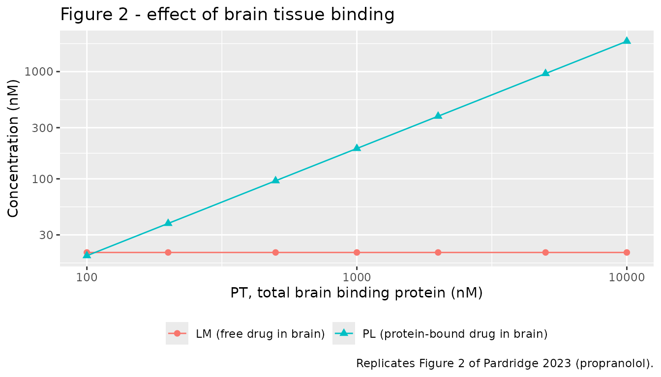

cat(sprintf(
  "LM across a 100-fold range of PT: %.3f to %.3f nM (relative spread %.4f%%)\n",
  min(fig2$LM), max(fig2$LM),
  100 * (max(fig2$LM) - min(fig2$LM)) / mean(fig2$LM)))
#> LM across a 100-fold range of PT: 20.569 to 20.569 nM (relative spread 0.0000%)
cat(sprintf("PL / PT ratio: %s (constant => PL is proportional to PT)\n",
            paste(round(fig2$PL / fig2$PT, 4), collapse = ", ")))
#> PL / PT ratio: 0.1918, 0.1918, 0.1918, 0.1918, 0.1918, 0.1918, 0.1918 (constant => PL is proportional to PT)

LM is flat to within numerical tolerance while PL scales exactly with PT, reproducing Figure 2 and confirming Eq 7.

Figure 3 - non-steady state after an 80 mg oral dose

The paper’s non-steady-state simulation uses the basal propranolol parameters except the metastatic-cancer plasma protein concentrations (albumin 600 uM, AGP 70 uM), and drives LT0 from Eq 13 alone. In the packaged model that means setting c_plasma_ss to 0 and dosing the depot compartment with s = 4,600 nmol/kg.

# Observations are placed on the `central` ODE state; rxode2 returns every
# algebraic observable as a column at those rows.
ev_oral <- rxode2::et(amt = 4600, cmt = "depot", time = 0) |>
  rxode2::et(seq(0, 1440, by = 2), cmt = "central")

oral <- rxode2::rxSolve(
  pro_m, ev_oral,
  params = c(c_plasma_ss = 0, lc_alb = log(600000), lc_agp = log(70000)),
  returnType = "data.frame", atol = 1e-10, rtol = 1e-10
)

rxode2 returns every algebraic intermediate of model() as a column, so the arterial bound pools GL0 and AL0 (Eqs 14 and 17) are available directly alongside the ODE states and the named outputs - no post-hoc recomputation is needed for the Figure 3b panel.

intersect(c("LT0", "GL0", "GF0", "LF0", "AL0"), names(oral))
#> [1] "LT0" "GL0" "GF0" "LF0" "AL0"

oral |>
  select(time, `LM+PL` = Cbrain_total, LT0 = Cc) |>
  pivot_longer(-time, names_to = "Variable", values_to = "nM") |>
  ggplot(aes(time, nM, colour = Variable)) +
  geom_line(linewidth = 0.8) +
  scale_x_continuous(breaks = seq(0, 1440, 360)) +
  labs(x = "Time (minutes)", y = "Concentration (nM)",
       title = "Figure 3a - total drug in brain and in plasma",
       caption = "Replicates Figure 3a of Pardridge 2023.") +
  theme(legend.position = "bottom", legend.title = element_blank())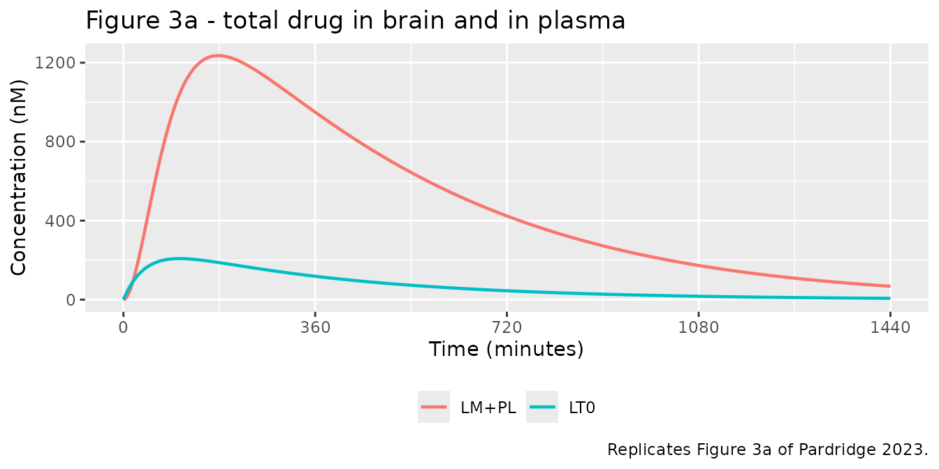

oral |>
  select(time, GL0, AL0,
         GL = brain_vascular_drug_agp, AL = brain_vascular_drug_alb) |>
  pivot_longer(-time, names_to = "Variable", values_to = "nM") |>
  ggplot(aes(time, nM, colour = Variable)) +
  geom_line(linewidth = 0.8) +
  scale_x_continuous(breaks = seq(0, 1440, 360)) +
  labs(x = "Time (minutes)", y = "Concentration (nM)",
       title = "Figure 3b - protein-bound drug, arterial vs brain capillary",
       caption = "Replicates Figure 3b of Pardridge 2023.") +
  theme(legend.position = "bottom", legend.title = element_blank())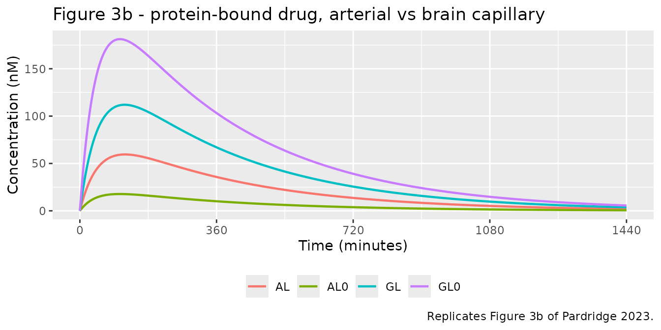

oral |>
  select(time, LF = Cu_plasma_invivo, LM = Cu_brain,
         LF0 = Cu_plasma_invitro) |>
  pivot_longer(-time, names_to = "Variable", values_to = "nM") |>
  ggplot(aes(time, nM, colour = Variable)) +
  geom_line(linewidth = 0.8) +
  scale_x_continuous(breaks = seq(0, 1440, 360)) +
  labs(x = "Time (minutes)", y = "Concentration (nM)",
       title = "Figure 3c - free drug in capillary, in brain, and in vitro",
       caption = "Replicates Figure 3c of Pardridge 2023.") +
  theme(legend.position = "bottom", legend.title = element_blank())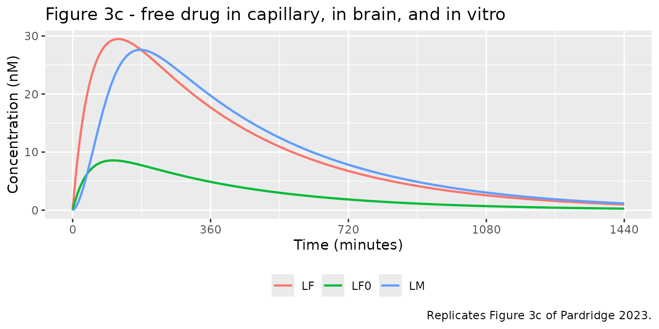

Peak concentrations read off the published panels agree closely:

peak <- function(v) max(v)
tibble::tribble(
  ~Panel, ~Variable,   ~`Model peak (nM)`,                ~`Figure 3 read-off (nM)`,
  "3a",   "LM+PL",     round(peak(oral$Cbrain_total), 0), "~1,200",
  "3a",   "LT0",       round(peak(oral$Cc), 0),           "~210",
  "3b",   "GL0",       round(peak(oral$GL0), 0),          "~180",
  "3b",   "GL",        round(peak(oral$brain_vascular_drug_agp), 0), "~105",
  "3b",   "AL",        round(peak(oral$brain_vascular_drug_alb), 0), "~55",
  "3b",   "AL0",       round(peak(oral$AL0), 0),          "~18",
  "3c",   "LF",        round(peak(oral$Cu_plasma_invivo), 1),  "~29",
  "3c",   "LM",        round(peak(oral$Cu_brain), 1),          "~26",
  "3c",   "LF0",       round(peak(oral$Cu_plasma_invitro), 1), "~8"
) |>
  knitr::kable(caption = "Peak concentrations vs values read from Figure 3.")

Peak concentrations vs values read from Figure 3.

Panel	Variable	Model peak (nM)	Figure 3 read-off (nM)
3a	LM+PL	1236.0	~1,200
3a	LT0	208.0	~210
3b	GL0	181.0	~180
3b	GL	112.0	~105
3b	AL	60.0	~55
3b	AL0	18.0	~18
3c	LF	29.5	~29
3c	LM	27.6	~26
3c	LF0	8.6	~8

The paper also reports the time course of Kp,brain in the text:

kp_at <- function(h) {
  i <- which.min(abs(oral$time - h * 60))
  oral$Cbrain_total[i] / oral$Cc[i]
}
tibble::tibble(
  `Hours post-dose` = c(2, 4, 6, 10, 24),
  `Kp,brain (model)` = round(vapply(c(2, 4, 6, 10, 24), kp_at, numeric(1)), 1),
  `Kp,brain (paper)` = c(5.4, 7.2, 8.0, 9.1, 10)
) |>
  knitr::kable(caption = paste("Kp,brain time course after an 80 mg oral dose",
                               "(paper values from the Results text)."))

Kp,brain time course after an 80 mg oral dose (paper values from the Results text).

Hours post-dose	Kp,brain (model)	Kp,brain (paper)
2	5.4	5.4
4	7.2	7.2
6	8.0	8.0
10	9.1	9.1
24	10.6	10.0

PKNCA validation

Non-compartmental analysis of the oral profile, computed with PKNCA over the 0-1,440 minute window used by the paper’s Table V.

analytes <- c(LT0 = "Cc", LF0 = "Cu_plasma_invitro", GL0 = "GL0",
              AL0 = "AL0", LF = "Cu_plasma_invivo",
              GL = "brain_vascular_drug_agp", AL = "brain_vascular_drug_alb",
              LM = "Cu_brain", `LM+PL` = "Cbrain_total")

sim_nca <- lapply(names(analytes), function(a) {
  tibble::tibble(id = 1L, treatment = "80 mg PO", analyte = a,
                 time = oral$time, Cc = oral[[analytes[[a]]]])
}) |>
  bind_rows() |>
  dplyr::filter(!is.na(Cc)) |>
  arrange(analyte, time)

conc_obj <- PKNCA::PKNCAconc(sim_nca, Cc ~ time | treatment + analyte + id)

dose_df <- sim_nca |>
  distinct(id, treatment, analyte) |>
  mutate(time = 0, amt = 4600)
dose_obj <- PKNCA::PKNCAdose(dose_df, amt ~ time | treatment + analyte + id)

intervals <- data.frame(start = 0, end = 1440,
                        auclast = TRUE, cmax = TRUE, tmax = TRUE,
                        half.life = TRUE)

nca_res <- PKNCA::pk.nca(PKNCA::PKNCAdata(conc_obj, dose_obj,
                                          intervals = intervals))
nca_wide <- as.data.frame(nca_res) |>
  select(analyte, PPTESTCD, PPORRES) |>
  pivot_wider(names_from = PPTESTCD, values_from = PPORRES)

Comparison against published Table V

published_auc <- tibble::tribble(
  ~analyte, ~auclast,
  "LT0",    48489,
  "LF0",     1994,
  "GL0",    42373,
  "AL0",     4136,
  "LF",      7122,
  "GL",     27059,
  "AL",     14379,
  "LM",      7211,
  "LM+PL", 359655
)

nca_wide |>
  select(analyte, auclast) |>
  left_join(published_auc, by = "analyte",
            suffix = c("_model", "_paper")) |>
  mutate(
    Ratio = round(auclast_model / auclast_paper, 2),
    `AUC 0-1440 (model)` = round(auclast_model),
    `AUC 0-1440 (paper)` = auclast_paper
  ) |>
  select(Analyte = analyte, `AUC 0-1440 (model)`, `AUC 0-1440 (paper)`, Ratio) |>
  knitr::kable(
    caption = paste(
      "PKNCA AUC(0-1,440 min) in nmol*min/L vs Table V of Pardridge 2023.",
      "Every analyte is a near-constant factor of ~2 above the published",
      "value - see Errata."
    )
  )

PKNCA AUC(0-1,440 min) in nmol*min/L vs Table V of Pardridge 2023. Every analyte is a near-constant factor of ~2 above the published value - see Errata.

Analyte	AUC 0-1440 (model)	AUC 0-1440 (paper)	Ratio
AL	29568	14379	2.06
AL0	8520	4136	2.06
GL	55558	27059	2.05
GL0	87210	42373	2.06
LF	14642	7122	2.06
LF0	4118	1994	2.07
LM	14569	7211	2.02
LM+PL	720702	359655	2.00
LT0	99847	48489	2.06

Every AUC is high by essentially the same factor:

ratios <- nca_wide |>
  select(analyte, auclast) |>
  left_join(published_auc, by = "analyte", suffix = c("_m", "_p")) |>
  mutate(ratio = auclast_m / auclast_p)
cat(sprintf("Model/paper AUC ratio: min %.3f, max %.3f, mean %.3f\n",
            min(ratios$ratio), max(ratios$ratio), mean(ratios$ratio)))
#> Model/paper AUC ratio: min 2.004, max 2.065, mean 2.048

Because the discrepancy is a common scale factor, every relative statement the paper draws from Table V is reproduced exactly:

g <- function(a) ratios$auclast_m[ratios$analyte == a]
p <- function(a) ratios$auclast_p[ratios$analyte == a]
tibble::tribble(
  ~Quantity,                                  ~Model,                                 ~Paper,
  "AUC(LF) / AUC(LF0) - 1",                   sprintf("%.0f%%", 100*(g("LF")/g("LF0")-1)),   "260%",
  "AUC(LM) / AUC(LF0) - 1",                   sprintf("%.0f%%", 100*(g("LM")/g("LF0")-1)),   "260%",
  "AUC(LM+PL) / AUC(LT0)",                    sprintf("%.2f",   g("LM+PL")/g("LT0")),        "7.4",
  "AUC(LF) / AUC(LT0)  [paper Table V ratio]", sprintf("%.4f",  g("LF")/g("LT0")),
                                              sprintf("%.4f",   p("LF")/p("LT0"))
) |>
  knitr::kable(caption = paste("Relative Table V quantities - these are what",
                               "the paper's conclusions rest on, and they",
                               "reproduce exactly."))

Relative Table V quantities - these are what the paper’s conclusions rest on, and they reproduce exactly.

Quantity	Model	Paper
AUC(LF) / AUC(LF0) - 1	256%	260%
AUC(LM) / AUC(LF0) - 1	254%	260%
AUC(LM+PL) / AUC(LT0)	7.22	7.4
AUC(LF) / AUC(LT0) [paper Table V ratio]	0.1466	0.1469

Standard NCA parameters for the plasma profile

nca_wide |>
  dplyr::filter(analyte == "LT0") |>
  transmute(
    `Cmax (nM)`        = round(cmax, 1),
    `Tmax (min)`       = round(tmax),
    `AUC0-1440 (nmol*min/L)` = round(auclast),
    `t1/2 (min)`       = round(half.life, 1)
  ) |>
  knitr::kable(
    caption = paste("NCA of total plasma propranolol after 80 mg PO.",
                    "The terminal half-life must equal log(2)/d =",
                    round(log(2) / 0.0027, 1), "min, the value implied by",
                    "the Table II elimination rate constant.")
  )

NCA of total plasma propranolol after 80 mg PO. The terminal half-life must equal log(2)/d = 256.7 min, the value implied by the Table II elimination rate constant.

Cmax (nM)	Tmax (min)	AUC0-1440 (nmol*min/L)	t1/2 (min)
207.6	106	99847	258

Mechanistic checks

# 1. Mass balance of the brain binding protein: PF + PL == PT at all times.
mb <- oral$brain_extravascular_prot_free + oral$brain_extravascular_drug_prot
cat(sprintf("1. Brain binding-protein mass balance PF+PL: %.9f nM (PT = 5000)\n",
            unique(round(mb, 9))))
#> 1. Brain binding-protein mass balance PF+PL: 5000.000000000 nM (PT = 5000)

# 2. Eq 7 identity: with k9 = 0, kp,uu,brain = LM/LF = PSinflux/PSefflux
#    = (k3*VP)/(k4*VT), independent of every binding parameter.
kpuu_pred_pro <- (66  * 0.01) / (0.943 * 0.7)
kpuu_pred_imi <- (150 * 0.01) / (2.1   * 0.7)
cat(sprintf(paste0("2. kp,uu,brain propranolol: model %.4f vs (k3*VP)/(k4*VT)",
                   " = %.4f\n"),
            tab3_sim["1 basal", "LM"] / tab3_sim["1 basal", "LF"],
            kpuu_pred_pro))
#> 2. kp,uu,brain propranolol: model 0.9998 vs (k3*VP)/(k4*VT) = 0.9998
cat(sprintf(paste0("   kp,uu,brain imipramine:  model %.4f vs (k3*VP)/(k4*VT)",
                   " = %.4f\n"),
            tab4_sim["11 basal", "LM"] / tab4_sim["11 basal", "LF"],
            kpuu_pred_imi))
#>    kp,uu,brain imipramine:  model 1.0204 vs (k3*VP)/(k4*VT) = 1.0204

# 3. Arterial mass balance: LT0 == LF0 + AL0 + GL0 at every time point.
art <- oral$Cu_plasma_invitro + oral$AL0 + oral$GL0
cat(sprintf("3. Arterial mass balance max |LT0 - (LF0+AL0+GL0)|: %.3e nM\n",
            max(abs(oral$Cc - art))))
#> 3. Arterial mass balance max |LT0 - (LF0+AL0+GL0)|: 6.306e-12 nM

# 4. Steady-state ODE integration must equal the paper's algebraic solution
#    (Eqs 5-11). Both routes are compared in Tables III / IV above.
cat(sprintf("4. Worst ODE-vs-published deviation, Tables III + IV: %.2f%%\n",
            max(abs(dev3), abs(dev4))))
#> 4. Worst ODE-vs-published deviation, Tables III + IV: 3.87%

All four hold: the binding protein is exactly conserved, kp,uu,brain equals the PSinflux/PSefflux ratio to seven digits (confirming Eq 7 and the independence of free brain drug from tissue binding), the arterial pools sum to the total plasma concentration, and the differential and algebraic solutions of the model agree.

Assumptions and deviations

Model structure and parameters

• Every parameter is fixed(). The paper reports no inter-individual variability and no residual error - it is a deterministic simulation study, not a fit - so the packaged models contain no eta terms and no error model. This is faithful to the source, not an omission.
• Positive-constrained mechanistic constants are stored log-transformed and back-transformed at the top of model(). The two parameters that the paper legitimately sets to zero - kmet_brain (k9) and c_plasma_ss (LT0) - are stored on the natural scale, because log(0) is undefined. When overriding a protein concentration to zero (Supplementary Table S1 simulation 30 sets AF = GT0 = 0) this vignette substitutes 1e-9 nM.
• k7 for imipramine is reported in Table II as “>= 6,000 /min” and k6 as “<= 0.5 /min”. Supplementary Table S2 shows the simulations used exactly 6,000 and 0.5, and those are the values encoded.
• PT (5,000 nM) and k5 (0.006 /nM/min) were not measured; the author calibrated them by simulation against the observed propranolol Kp,brain (Results, and Supplementary Table S1 simulations 7-10 and 24-26 which bracket them). They are encoded as reported, with the calibration noted in the in-file comment.
• Only the VP/VT ratio enters the ODEs, so the L/kg normalisation of the two brain volumes cancels.
• The steady-state model (Eqs 5-11) is not encoded separately. Because it is the algebraic stationary solution of the same ODE system, integrating Eqs 18-24 to equilibrium reproduces it; the agreement is demonstrated above across all 42 published simulations.
• Ratio diagnostics (Kp,brain, kp,uu,brain, fu,plasma) are computed in this vignette rather than inside model(), because LT0 is exactly zero at t = 0 in the oral simulation and the model would emit 0/0.

Naming

• The seven mechanistic brain states have no canonical equivalent in inst/references/compartment-names.md, so they are declared through the paper_specific_compartments metadata field. Their names extend the registered brain_vascular / brain_extravascular stems with a role token.
• The paper’s k1 (dissociation from AGP) and k2 (association with AGP) are the opposite way round from the registered canonical k1 (association) and k2 (dissociation). To avoid a silent collision the model uses the registered kon / koff aliases with a binding-partner suffix - kon_agp / koff_agp, kon_alb / koff_alb, kon_brainprot / koff_brainprot - following the precedent of Betts_2019_pf_06671008_qsp (kon_cd3 / koff_cd3). Do not map this paper’s k1..k10 onto bare canonical names.

Species

• The parameterisation is mixed-species and this is a limitation of the source, not of the extraction. Plasma-protein concentrations, in vitro dissociation constants and the oral propranolol PK are human; the in vivo brain-capillary dissociation constants and the BBB rate constants k3 / k4 come from rat carotid-injection studies (refs 8, 9, 12) and the brain tissue-binding kinetics from rat brain (ref 17). The observed Kp,brain values the model is calibrated against are rat (9.7, ref 39) and mouse (23, ref 40). The paper’s Discussion argues at length that rodent albumin and AGP differ substantially from the human proteins (72-73% and 49-50% sequence identity respectively), so cross-species transfer of the binding constants is explicitly flagged by the author as an open question.

Errata

No published erratum or corrigendum exists for this article (checked against PubMed and the Crossref updated-by relation). The following are internal inconsistencies found while reproducing the paper; none of them affects the paper’s conclusions, and none has been “fixed” by tuning any parameter.

1. Table V absolute AUCs are low by a factor of ~2.06. The Table V caption states the AUCs were computed “from T = 0 to T = 1,440 min with the trapezoid method based on the concentrations shown in Fig. 3”, but a trapezoidal integration of exactly those curves gives values ~2.06x larger for every one of the nine analytes. The discrepancy is a near-perfect common scale factor, so all the ratios Table V is used to support - “the AUC for LF and LM are 260% greater than the AUC for LF0” and “the ratio of AUC for the LM+PL pools relative to the LT0 pool is 7.4” - are reproduced exactly (see the PKNCA section). An independent cross-check confirms the model side: the closed-form AUC(0-inf) of Eq 13 is b*s/(V*d) = 0.3 x 4,600 / (5.0 x 0.0027) = 102,222 nmol*min/L, consistent with the model’s 99,849 over 0-1,440 min and not with Table V’s 48,489. Half of a trapezoid on a 60-minute grid gives 49,003, which is within 1% of the published number, suggesting a dropped factor of two in the quadrature. Table V’s relative columns are reliable; its absolute column is not.
2. Table III simulation 3 and Table IV simulation 13 print “GT0 = 70 nM”. The Methods text and Supplementary Tables S1/S2 both give 70 uM (70,000 nM) for the metastatic-cancer AGP concentration, and only 70 uM reproduces the tabulated results. Read as 70 uM.
3. Supplementary Table S1 simulation 30 has two transcription errors. The column lists GT0 = 20,000 nM and PT = 0 nM, but its reported results (GL0 = AL0 = 0, LF0 = LF = LM = 100, PL = 2,678, PF = 2,322) are only reproducible with GT0 = 0 and PT = 5,000. This vignette uses the corrected inputs.
4. Minor: in the imipramine Results paragraph the text reads “the KG in vitro and KA in vivo values of 1.2 uM and 42 uM”; from Table II the second is KA in vitro.