Polymyxin B in obese patients (Wang 2021)
Source:vignettes/articles/Wang_2021_polymyxinB.Rmd
Wang_2021_polymyxinB.RmdModel and source
- Citation: Wang P, Zhang Q, Feng M, Sun T, Yang J, Zhang X. Population Pharmacokinetics of Polymyxin B in Obese Patients for Resistant Gram-Negative Infections. Front Pharmacol. 2021;12:754844. doi:10.3389/fphar.2021.754844. PMCID PMC8645997.
- Description: Two-compartment intravenous population PK model for polymyxin B (sum of polymyxin B1 and B2) in obese Chinese adults (BMI >= 30) with resistant Gram-negative infections, sampled at steady state (Wang 2021). No covariate was retained: age, total, ideal and adjusted body weight, BMI, sex, SOFA score, three creatinine clearance estimates, serum creatinine and GFR were screened and rejected. Log-normal inter-individual variability on CL, V2 and Q (none on V); proportional residual error.
- Article: Front Pharmacol 2021;12:754844
Wang et al. fitted a two-compartment population PK model to 142 steady-state plasma polymyxin B concentrations (polymyxin B1 + B2) from 26 obese adults. No covariate was retained, including the three body-size descriptors (total, ideal and adjusted body weight). The paper then used Monte Carlo simulation to compare fixed and weight-based dosing regimens against an exposure window of AUCss,24h 50-100 mg*h/L (Table 3, Figure 4). That table is the validation target of this article.
Population
The analysis included 26 adults (17 male, 9 female; median age 52 years, range 18-83) with BMI >= 30 (median 32.65, range 30.04-40.35) treated with intravenous polymyxin B for multidrug-resistant Gram-negative infections at the First Affiliated Hospital of Zhengzhou University, China, between April 2018 and March 2021 (Table 1). Total body weight was 75-125 kg (median 90), ideal body weight 48.76-74.99 kg and adjusted body weight 59.26-92.82 kg. Cockcroft-Gault creatinine clearance ranged from 21.35 to 239.99 mL/min; CRRT and ECMO were exclusion criteria. Patients received a 100-200 mg loading dose followed by 50-100 mg twice daily, infused over at least 1 h. Ten patients contributed 4-7 samples within one dosing interval on day 4 and 16 contributed two routine TDM samples (pre-dose and 2 h).
The same information is available programmatically via
readModelDb("Wang_2021_polymyxinB")()$population.
Source trace
| Equation / parameter | Value | Source location |
|---|---|---|
lvc (V) |
log(11.24 L) | Table 2, tvV |
lvp (V2) |
log(39.70 L) | Table 2, tvV2 |
lcl (CL) |
log(2.86 L/h) | Table 2, tvCL |
lq (Q) |
log(7.36 L/h) | Table 2, tvQ |
etalcl |
0.17 (variance) | Table 2, omega^2 CL |
etalvp |
1.00 (variance) | Table 2, omega^2 V2 |
etalq |
0.43 (variance) | Table 2, omega^2 Q |
| no IIV on V | – | Results: V random effect dropped (shrinkage > 0.5) |
propSd |
0.24 | Table 2, stdev0; Results (‘proportional error model’) |
two-compartment ODE, IV infusion into central
|
n/a | Results, ‘Population PK Model’; Methods (infusion >= 1 h) |
| covariates | none | Results: no systematic relationship for any of the 12 screened covariates |
Virtual cohort and regimens
The paper simulated 1,000 subjects for each of 23 regimens on the fourth day of therapy (Methods, ‘Monte Carlo Simulations’): five fixed regimens (a loading dose of twice the maintenance dose, then 50-150 mg every 12 h) and six weight-based regimens (2.5 mg/kg loading dose, then 1.25 or 1.5 mg/kg every 12 h) evaluated at the 10th, 50th and 90th percentiles of total, adjusted and ideal body weight. All doses were infused at 50 mg/h.
Here each regimen is given the same 200 virtual patients (common random numbers). Because the model has no covariates, a virtual patient is just a set of three random effects. They are drawn with base R’s random number generator as a Latin hypercube (one draw per 1/200 probability stratum of each random effect) and passed to the model as data, with the model’s own random effects switched off. The cohort, and every number below, is therefore identical on every machine and every rxode2 build.
mod <- readModelDb("Wang_2021_polymyxinB")
ui <- rxode2::rxode(mod)
#> ℹ parameter labels from comments will be replaced by 'label()'
omega <- ui$omega

n_sub <- 200L
set.seed(2021)
lhs_eta <- function(n, variance) {
  qnorm((sample.int(n) - 0.5) / n) * sqrt(variance)
}
etas <- data.frame(
  subj = seq_len(n_sub),
  etalcl = lhs_eta(n_sub, omega["etalcl", "etalcl"]),
  etalvp = lhs_eta(n_sub, omega["etalvp", "etalvp"]),
  etalq = lhs_eta(n_sub, omega["etalq", "etalq"])
)

# Table 3 regimens. The weight is the body weight used to compute the mg/kg
# doses; fixed regimens have none.
regimens <- dplyr::bind_rows(
  tibble(
    scheme = "Fixed",
    weight = NA_real_,
    ld = c(100, 150, 200, 250, 300),
    md = c(50, 75, 100, 125, 150)
  ),
  tidyr::expand_grid(
    md_mgkg = c(1.25, 1.5),
    tibble::tribble(
      ~scale, ~weight,
      "TBW", 75, "TBW", 90, "TBW", 120,
      "ABW", 62, "ABW", 76, "ABW", 89,
      "IBW", 51, "IBW", 66, "IBW", 70
    )
  ) |>
    dplyr::mutate(
      scheme = paste0("2.5 mg/kg + ", md_mgkg, " mg/kg q12h; ", scale),
      ld = 2.5 * weight,
      md = md_mgkg * weight
    )
) |>
  dplyr::mutate(
    regimen = ifelse(
      scheme == "Fixed",
      paste0(ld, " mg + ", md, " mg q12h"),
      paste0(scheme, " ", weight, " kg")
    ),
    arm = dplyr::row_number()
  ) |>
  dplyr::select(arm, regimen, scheme, weight, ld, md)
stopifnot(nrow(regimens) == 23L, !anyDuplicated(regimens$regimen))

infusion_rate <- 50 # mg/h (Methods)
dose_times <- seq(0, 84, by = 12) # loading dose at 0, maintenance through day 4

make_arm <- function(arm, regimen, ld, md, id_offset, dense = FALSE) {
  amt <- c(ld, rep(md, length(dose_times) - 1L))
  doses <- tibble(time = dose_times, amt = amt, rate = infusion_rate, evid = 1L)
  obs_times <- if (dense) {
    # Day 1 (for the first-24-h PTA) and day 4 (72-96 h), plus the exact end
    # of every infusion so the trapezoid catches each peak.
    sort(unique(c(
      seq(0, 24, by = 0.25),
      seq(72, 96, by = 0.25),
      (dose_times + amt / infusion_rate)[dose_times < 24 | dose_times >= 72]
    )))
  } else {
    c(0, 24, 72, 96)
  }
  obs <- tibble(time = obs_times, amt = NA_real_, rate = NA_real_, evid = 0L)
  one <- dplyr::bind_rows(doses, obs) |>
    dplyr::mutate(cmt = "central")
  tidyr::expand_grid(etas, one) |>
    dplyr::mutate(id = id_offset + subj, arm = arm, regimen = regimen) |>
    dplyr::arrange(id, time, dplyr::desc(evid))
}

make_events <- function(regs, dense = FALSE, id_base = 0L) {
  lapply(seq_len(nrow(regs)), function(i) {
    r <- regs[i, ]
    make_arm(r$arm, r$regimen, r$ld, r$md,
             id_offset = id_base + (i - 1L) * n_sub, dense = dense)
  }) |>
    dplyr::bind_rows()
}

events <- make_events(regimens)
stopifnot(
  !anyDuplicated(unique(events[, c("id", "time", "evid")])),
  dplyr::n_distinct(events$id) == 23L * n_sub
)
Simulation
The paper’s exposure metrics are areas under the curve over day 1
(0-24 h) and day 4 (72-96 h). For the 23-regimen table they are read
from an integrated-concentration state appended to the model in this
article (d/dt(AUC) <- Cc), which is exact and cheap;
PKNCA is used below to confirm that state against a trapezoidal NCA on a
dense sampling grid.
mod_auc <- rxode2::zeroRe(mod) |>
  rxode2::model(d/dt(AUC) <- Cc, append = TRUE)
#> ℹ parameter labels from comments will be replaced by 'label()'

solve_fixed_eta <- function(model, ev, ...) {
  withCallingHandlers(
    rxode2::rxSolve(model, events = ev, omega = NA, returnType = "data.frame", ...),
    warning = function(w) {
      if (grepl("without 'omega'", conditionMessage(w))) {
        invokeRestart("muffleWarning")
      }
    }
  )
}
auc_windows <- function(sim_df) {
  sim_df |>
    dplyr::group_by(id, regimen) |>
    dplyr::summarise(
      auc_day1 = AUC[time == 24] - AUC[time == 0],
      auc_day4 = AUC[time == 96] - AUC[time == 72],
      .groups = "drop"
    )
}

sim <- solve_fixed_eta(mod_auc, events, keep = c("arm", "regimen"))

# The random effects came from the data: clearance must vary across subjects
# and must equal exp(lcl + etalcl) for each of them.
cl_check <- sim |>
  dplyr::distinct(id, cl) |>
  dplyr::mutate(subj = (id - 1L) %% n_sub + 1L) |>
  dplyr::left_join(etas, by = "subj")
stopifnot(
  dplyr::n_distinct(round(cl_check$cl, 8)) == n_sub,
  max(abs(cl_check$cl / (2.86 * exp(cl_check$etalcl)) - 1)) < 1e-10
)

auc <- auc_windows(sim) |>
  dplyr::left_join(regimens, by = "regimen")
stopifnot(nrow(auc) == 23L * n_sub, !anyNA(auc$auc_day1), !anyNA(auc$auc_day4))
PKNCA check of the exposure metric
The five fixed regimens are re-simulated on a dense grid (every 15 minutes over days 1 and 4, plus each infusion end) and the day-1 and day-4 AUCs are computed with PKNCA, one regimen at a time.
fixed_regs <- regimens |> dplyr::filter(scheme == "Fixed")
events_dense <- make_events(fixed_regs, dense = TRUE)
sim_dense <- solve_fixed_eta(mod_auc, events_dense, keep = c("regimen"))

nca_one <- function(reg) {
  conc <- sim_dense |>
    dplyr::filter(regimen == reg, !is.na(Cc)) |>
    dplyr::mutate(Cc = pmax(Cc, 0)) |>
    dplyr::select(id, time, Cc, regimen)
  doses <- events_dense |>
    dplyr::filter(regimen == reg, evid == 1L) |>
    dplyr::mutate(duration = amt / rate) |>
    dplyr::select(id, time, amt, duration, regimen)
  res <- PKNCA::pk.nca(PKNCA::PKNCAdata(
    PKNCA::PKNCAconc(conc, Cc ~ time | regimen + id),
    PKNCA::PKNCAdose(doses, amt ~ time | regimen + id,
                     route = "intravascular", duration = "duration"),
    intervals = data.frame(start = c(0, 72), end = c(24, 96), auclast = TRUE)
  ))
  as.data.frame(res)
}
nca_res <- lapply(fixed_regs$regimen, nca_one) |>
  dplyr::bind_rows() |>
  dplyr::filter(PPTESTCD == "auclast") |>
  dplyr::mutate(window = ifelse(start == 0, "pknca_day1", "pknca_day4")) |>
  dplyr::select(id, regimen, window, PPORRES) |>
  tidyr::pivot_wider(names_from = window, values_from = PPORRES)

nca_vs_ode <- nca_res |>
  dplyr::inner_join(auc_windows(sim_dense), by = c("id", "regimen"))
stopifnot(nrow(nca_vs_ode) == 5L * n_sub)

nca_vs_ode |>
  dplyr::group_by(regimen) |>
  dplyr::summarise(
    # Computed first: summarise() evaluates in order, and the medians below
    # overwrite pknca_day4.
    max_rel_diff_pct = 100 * max(abs(c(pknca_day1 / auc_day1, pknca_day4 / auc_day4) - 1)),
    pknca_day4 = median(pknca_day4),
    ode_day4 = median(auc_day4),
    .groups = "drop"
  ) |>
  dplyr::relocate(max_rel_diff_pct, .after = ode_day4) |>
  dplyr::rename(
    "Regimen" = regimen,
    "Median day-4 AUC, PKNCA (mg*h/L)" = pknca_day4,
    "Median day-4 AUC, ODE state (mg*h/L)" = ode_day4,
    "Max per-subject difference (%)" = max_rel_diff_pct
  ) |>
knitr::kable(digits = 2)| Regimen | Median day-4 AUC, PKNCA (mg*h/L) | Median day-4 AUC, ODE state (mg*h/L) | Max per-subject difference (%) |
|---|---|---|---|
| 100 mg + 50 mg q12h | 32.75 | 32.76 | 0.21 |
| 150 mg + 75 mg q12h | 49.12 | 49.14 | 0.16 |
| 200 mg + 100 mg q12h | 65.49 | 65.51 | 0.12 |
| 250 mg + 125 mg q12h | 81.86 | 81.88 | 0.10 |
| 300 mg + 150 mg q12h | 98.23 | 98.24 | 0.09 |
# PKNCA linear-up/log-down trapezoid on a 15-min grid against the exact integral.
# Deterministic; measured maximum 0.21%.
stopifnot(
  max(abs(nca_vs_ode$pknca_day1 / nca_vs_ode$auc_day1 - 1)) < 0.005,
  max(abs(nca_vs_ode$pknca_day4 / nca_vs_ode$auc_day4 - 1)) < 0.005
)
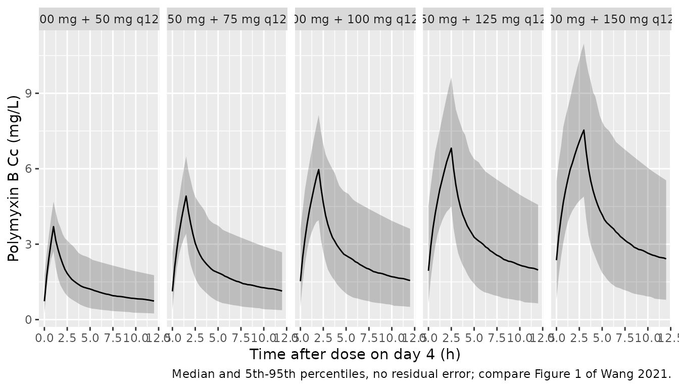
The day-4 concentration profiles of the fixed regimens, for comparison with the steady-state observations in Figure 1 of the paper (1-h infusions of 50-100 mg; here the Table 3 regimens at 50 mg/h):
sim_dense |>
  dplyr::filter(time >= 72, time <= 84, !is.na(Cc)) |>
  dplyr::group_by(regimen, time) |>
  dplyr::summarise(
    Q05 = quantile(Cc, 0.05), Q50 = median(Cc), Q95 = quantile(Cc, 0.95),
    .groups = "drop"
  ) |>
  dplyr::mutate(regimen = factor(regimen, levels = fixed_regs$regimen)) |>
  ggplot(aes(time - 72, Q50)) +
  geom_ribbon(aes(ymin = Q05, ymax = Q95), alpha = 0.25) +
  geom_line() +
  facet_wrap(~regimen, nrow = 1) +
  labs(
    x = "Time after dose on day 4 (h)",
    y = "Polymyxin B Cc (mg/L)",
    caption = "Median and 5th-95th percentiles, no residual error; compare Figure 1 of Wang 2021."
  )
Replicate Figure 4: day-4 exposure by regimen
auc |>
  dplyr::mutate(
    panel = ifelse(scheme == "Fixed", "A: fixed regimens", "B: body-weight-based regimens"),
    regimen = factor(regimen, levels = regimens$regimen)
  ) |>
  ggplot(aes(regimen, auc_day4)) +
  geom_violin(draw_quantiles = c(0.25, 0.5, 0.75), scale = "width") +
  geom_hline(yintercept = c(50, 100), colour = "red", linetype = "dashed") +
  facet_grid(~panel, scales = "free_x", space = "free_x") +
  labs(
    x = NULL,
    y = "AUCss,24h on day 4 (mg*h/L)",
    caption = "Replicates Figure 4 of Wang 2021 (200 virtual patients per regimen)."
  ) +
  theme(axis.text.x = element_text(angle = 60, hjust = 1, size = 7))
#> Warning: The `draw_quantiles` argument of `geom_violin()` is deprecated as of ggplot2
#> 4.0.0.
#> ℹ Please use the `quantiles.linetype` argument instead.
#> This warning is displayed once per session.
#> Call `lifecycle::last_lifecycle_warnings()` to see where this warning was
#> generated.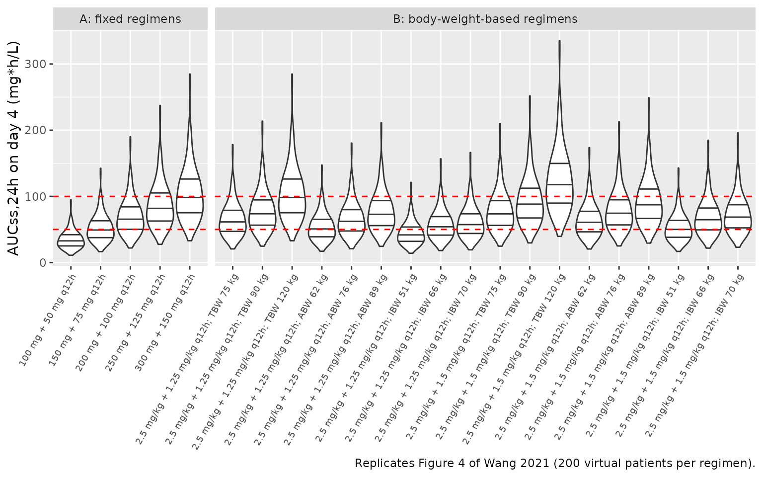
Replicate Table 3: target attainment
Table 3 gives, for each regimen, the probability that the day-4 AUCss,24h lies in the 50-100 mgh/L target window, the probability that it exceeds 100 mgh/L (toxicity), and the probability of target attainment (PTA) for a total-drug AUC0-24/MIC > 50 over the first 24 h of treatment, across MICs of 0.125-8 mg/L.
mics <- c(0.125, 0.25, 0.5, 1, 2, 4, 8)
sim_tab <- dplyr::bind_rows(
  auc |>
    dplyr::group_by(arm, regimen) |>
    dplyr::summarise(
      target = 100 * mean(auc_day4 >= 50 & auc_day4 <= 100),
      toxicity = 100 * mean(auc_day4 > 100),
      .groups = "drop"
    ) |>
    tidyr::pivot_longer(c(target, toxicity), names_to = "quantity", values_to = "simulated"),
  auc |>
    tidyr::crossing(mic = mics) |>
    dplyr::group_by(arm, regimen, mic) |>
    dplyr::summarise(simulated = 100 * mean(auc_day1 / mic > 50), .groups = "drop") |>
    dplyr::mutate(quantity = paste0("pta_", mic)) |>
    dplyr::select(-mic)
)

# Wang 2021 Table 3, in the row order of `regimens`. The paper labels the
# fourth and fifth fixed rows '200 mg + 125 mg' and '200 mg + 150 mg'; the
# Methods give 250 mg and 300 mg loading doses, and the PTA columns reproduce
# only with 250 mg and 300 mg (see Assumptions and deviations).
published <- tibble::tribble(
  ~target, ~toxicity, ~pta_0.125, ~pta_0.25, ~pta_0.5, ~pta_1, ~pta_2, ~pta_4, ~pta_8,
  13.0, 0.2, 100, 98.5, 74.7, 13.8, 0, 0, 0,
  43.6, 4.4, 100, 100, 95.4, 47.5, 2.7, 0, 0,
  59.8, 13.5, 100, 100, 98.5, 72.0, 11.9, 0, 0,
  60.6, 28.6, 100, 100, 99.4, 87.7, 27.4, 0.2, 0,
  46.6, 47.7, 100, 100, 19.9, 93.2, 45.5, 3.7, 0,
  59.0, 11.1, 100, 100, 97.9, 69.3, 10.5, 0, 0,
  59.2, 23.1, 100, 100, 99.1, 81.5, 22.1, 0, 0,
  46.7, 48.1, 100, 100, 100, 95.9, 47.8, 2.6, 0,
  47.3, 4.9, 100, 100, 96.1, 52.1, 4.4, 0, 0,
  55.9, 12.9, 100, 100, 98.3, 69.4, 11.4, 0, 0,
  62.8, 19.9, 100, 100, 99.2, 81.5, 17.1, 0, 0,
  31.1, 1.3, 100, 99.9, 90.9, 33.4, 0.6, 0, 0,
  50.1, 5.3, 100, 99.9, 95.4, 58.4, 5.1, 0, 0,
  56.5, 7.5, 100, 100, 97.3, 63.9, 6.0, 0, 0,
  61.9, 21.9, 100, 100, 98.6, 73.4, 13.0, 0, 0,
  53.1, 38.2, 100, 100, 99.4, 83.9, 25.5, 0.2, 0,
  34.0, 64.5, 100, 100, 100, 94.9, 51.0, 2.0, 0,
  58.4, 10.5, 100, 100, 96.7, 58.1, 6.0, 0, 0,
  59.4, 22.6, 100, 100, 98.7, 74.4, 14.4, 0, 0,
  55.8, 36.2, 100, 100, 99.6, 84.2, 22.2, 0, 0,
  45.7, 4.2, 100, 99.9, 92.4, 38.3, 1.0, 0, 0,
  57.7, 13.3, 100, 99.9, 97.0, 62.9, 6.7, 0, 0,
  64.4, 15.3, 100, 100, 98.2, 68.5, 8.1, 0, 0
) |>
  dplyr::mutate(arm = dplyr::row_number()) |>
  tidyr::pivot_longer(-arm, names_to = "quantity", values_to = "published")
stopifnot(nrow(published) == 23L * 9L)

cmp <- dplyr::inner_join(sim_tab, published, by = c("arm", "quantity")) |>
  dplyr::mutate(
    diff = simulated - published,
    # The one cell that is not a model disagreement: Table 3 prints 19.9% PTA
    # at MIC 0.5 for the 300 + 150 mg regimen, between 100% at MIC 0.25 and
    # 93.2% at MIC 1. PTA cannot rise with MIC, so the cell is a typesetting
    # error and is excluded from the gate below.
    known_misprint = arm == 5L & quantity == "pta_0.5"
  )
stopifnot(nrow(cmp) == 23L * 9L, sum(cmp$known_misprint) == 1L)

cmp |>
  dplyr::mutate(cell = sprintf("%.1f (%.1f)", simulated, published)) |>
  dplyr::select(regimen, quantity, cell) |>
  tidyr::pivot_wider(names_from = quantity, values_from = cell) |>
  dplyr::rename(
    "Regimen" = regimen,
    "Target AUC %" = target,
    "Toxicity %" = toxicity,
    "PTA MIC 0.125" = pta_0.125,
    "PTA MIC 0.25" = pta_0.25,
    "PTA MIC 0.5" = pta_0.5,
    "PTA MIC 1" = pta_1,
    "PTA MIC 2" = pta_2,
    "PTA MIC 4" = pta_4,
    "PTA MIC 8" = pta_8
  ) |>
knitr::kable(caption = "Simulated (published) percentages; published values are Table 3 of Wang 2021.")| Regimen | Target AUC % | Toxicity % | PTA MIC 0.125 | PTA MIC 0.25 | PTA MIC 0.5 | PTA MIC 1 | PTA MIC 2 | PTA MIC 4 | PTA MIC 8 |
|---|---|---|---|---|---|---|---|---|---|
| 100 mg + 50 mg q12h | 12.0 (13.0) | 0.0 (0.2) | 100.0 (100.0) | 100.0 (98.5) | 78.0 (74.7) | 12.5 (13.8) | 0.0 (0.0) | 0.0 (0.0) | 0.0 (0.0) |
| 150 mg + 75 mg q12h | 47.0 (43.6) | 2.5 (4.4) | 100.0 (100.0) | 100.0 (100.0) | 96.5 (95.4) | 46.0 (47.5) | 1.0 (2.7) | 0.0 (0.0) | 0.0 (0.0) |
| 200 mg + 100 mg q12h | 63.5 (59.8) | 12.0 (13.5) | 100.0 (100.0) | 100.0 (100.0) | 100.0 (98.5) | 75.0 (72.0) | 11.0 (11.9) | 0.0 (0.0) | 0.0 (0.0) |
| 250 mg + 125 mg q12h | 57.0 (60.6) | 30.5 (28.6) | 100.0 (100.0) | 100.0 (100.0) | 100.0 (99.4) | 89.5 (87.7) | 28.0 (27.4) | 0.0 (0.2) | 0.0 (0.0) |
| 300 mg + 150 mg q12h | 46.5 (46.6) | 49.5 (47.7) | 100.0 (100.0) | 100.0 (100.0) | 100.0 (19.9) | 95.5 (93.2) | 43.5 (45.5) | 1.0 (3.7) | 0.0 (0.0) |
| 2.5 mg/kg + 1.25 mg/kg q12h; TBW 75 kg | 60.5 (59.0) | 9.5 (11.1) | 100.0 (100.0) | 100.0 (100.0) | 100.0 (97.9) | 68.0 (69.3) | 9.0 (10.5) | 0.0 (0.0) | 0.0 (0.0) |
| 2.5 mg/kg + 1.25 mg/kg q12h; TBW 90 kg | 62.5 (59.2) | 20.5 (23.1) | 100.0 (100.0) | 100.0 (100.0) | 100.0 (99.1) | 85.0 (81.5) | 18.5 (22.1) | 0.0 (0.0) | 0.0 (0.0) |
| 2.5 mg/kg + 1.25 mg/kg q12h; TBW 120 kg | 46.5 (46.7) | 49.5 (48.1) | 100.0 (100.0) | 100.0 (100.0) | 100.0 (100.0) | 95.5 (95.9) | 43.5 (47.8) | 1.0 (2.6) | 0.0 (0.0) |
| 2.5 mg/kg + 1.25 mg/kg q12h; ABW 62 kg | 47.5 (47.3) | 3.5 (4.9) | 100.0 (100.0) | 100.0 (100.0) | 97.5 (96.1) | 51.0 (52.1) | 1.5 (4.4) | 0.0 (0.0) | 0.0 (0.0) |
| 2.5 mg/kg + 1.25 mg/kg q12h; ABW 76 kg | 62.0 (55.9) | 9.5 (12.9) | 100.0 (100.0) | 100.0 (100.0) | 100.0 (98.3) | 69.5 (69.4) | 9.0 (11.4) | 0.0 (0.0) | 0.0 (0.0) |
| 2.5 mg/kg + 1.25 mg/kg q12h; ABW 89 kg | 62.5 (62.8) | 20.0 (19.9) | 100.0 (100.0) | 100.0 (100.0) | 100.0 (99.2) | 84.0 (81.5) | 17.5 (17.1) | 0.0 (0.0) | 0.0 (0.0) |
| 2.5 mg/kg + 1.25 mg/kg q12h; IBW 51 kg | 31.5 (31.1) | 1.0 (1.3) | 100.0 (100.0) | 100.0 (99.9) | 92.0 (90.9) | 31.0 (33.4) | 0.0 (0.6) | 0.0 (0.0) | 0.0 (0.0) |
| 2.5 mg/kg + 1.25 mg/kg q12h; IBW 66 kg | 54.0 (50.1) | 5.0 (5.3) | 100.0 (100.0) | 100.0 (99.9) | 98.5 (95.4) | 55.0 (58.4) | 3.5 (5.1) | 0.0 (0.0) | 0.0 (0.0) |
| 2.5 mg/kg + 1.25 mg/kg q12h; IBW 70 kg | 56.0 (56.5) | 6.5 (7.5) | 100.0 (100.0) | 100.0 (100.0) | 99.5 (97.3) | 62.0 (63.9) | 6.0 (6.0) | 0.0 (0.0) | 0.0 (0.0) |
| 2.5 mg/kg + 1.5 mg/kg q12h; TBW 75 kg | 62.5 (61.9) | 20.0 (21.9) | 100.0 (100.0) | 100.0 (100.0) | 100.0 (98.6) | 74.5 (73.4) | 11.0 (13.0) | 0.0 (0.0) | 0.0 (0.0) |
| 2.5 mg/kg + 1.5 mg/kg q12h; TBW 90 kg | 54.5 (53.1) | 38.0 (38.2) | 100.0 (100.0) | 100.0 (100.0) | 100.0 (99.4) | 87.0 (83.9) | 23.0 (25.5) | 0.0 (0.2) | 0.0 (0.0) |
| 2.5 mg/kg + 1.5 mg/kg q12h; TBW 120 kg | 32.5 (34.0) | 66.0 (64.5) | 100.0 (100.0) | 100.0 (100.0) | 100.0 (100.0) | 97.5 (94.9) | 49.5 (51.0) | 1.5 (2.0) | 0.0 (0.0) |
| 2.5 mg/kg + 1.5 mg/kg q12h; ABW 62 kg | 61.0 (58.4) | 8.0 (10.5) | 100.0 (100.0) | 100.0 (100.0) | 98.5 (96.7) | 55.0 (58.1) | 3.0 (6.0) | 0.0 (0.0) | 0.0 (0.0) |
| 2.5 mg/kg + 1.5 mg/kg q12h; ABW 76 kg | 61.5 (59.4) | 21.5 (22.6) | 100.0 (100.0) | 100.0 (100.0) | 100.0 (98.7) | 76.0 (74.4) | 11.5 (14.4) | 0.0 (0.0) | 0.0 (0.0) |
| 2.5 mg/kg + 1.5 mg/kg q12h; ABW 89 kg | 54.5 (55.8) | 37.0 (36.2) | 100.0 (100.0) | 100.0 (100.0) | 100.0 (99.6) | 86.5 (84.2) | 22.5 (22.2) | 0.0 (0.0) | 0.0 (0.0) |
| 2.5 mg/kg + 1.5 mg/kg q12h; IBW 51 kg | 47.0 (45.7) | 3.0 (4.2) | 100.0 (100.0) | 100.0 (99.9) | 94.0 (92.4) | 34.0 (38.3) | 0.0 (1.0) | 0.0 (0.0) | 0.0 (0.0) |
| 2.5 mg/kg + 1.5 mg/kg q12h; IBW 66 kg | 61.5 (57.7) | 12.0 (13.3) | 100.0 (100.0) | 100.0 (99.9) | 99.5 (97.0) | 61.5 (62.9) | 6.0 (6.7) | 0.0 (0.0) | 0.0 (0.0) |
| 2.5 mg/kg + 1.5 mg/kg q12h; IBW 70 kg | 64.0 (64.4) | 15.0 (15.3) | 100.0 (100.0) | 100.0 (100.0) | 100.0 (98.2) | 66.5 (68.5) | 7.5 (8.1) | 0.0 (0.0) | 0.0 (0.0) |
gate <- cmp |> dplyr::filter(!known_misprint)
gate_summary <- c(
  p90_abs_diff = unname(quantile(abs(gate$diff), 0.9)),
  median_abs_diff_target_tox = median(abs(gate$diff[gate$quantity %in% c("target", "toxicity")])),
  median_abs_diff_pta_1 = median(abs(gate$diff[gate$quantity == "pta_1"]))
)
round(gate_summary, 2)
#>               p90_abs_diff median_abs_diff_target_tox
#>                        2.8                        1.4
#>      median_abs_diff_pta_1
#>                        2.0

# The cohort is drawn with base R and passed as data, so these numbers do not
# depend on the rxode2 build or thread count. Measured 2.8 / 1.4 / 2.0 points.
# Most PTA cells are trivially 0 or 100, so the gate looks at the informative
# ones. The paper's own 1,000-subject draw carries about 1.5 points of Monte
# Carlo error per cell and this 200-subject cohort a little more, which the
# bounds allow for. Mutations of the model measured against the same gate:
#   CL 15% too high                     6.6 target/toxicity, 7.4 MIC-1 PTA
#   omega^2 read as SD (variance ^ 2)  15.0 target/toxicity, 15.8 p90
#   no IIV on V2 and Q                  4.4 target/toxicity, 12.1 MIC-1 PTA
stopifnot(
  gate_summary[["p90_abs_diff"]] < 5,
  gate_summary[["median_abs_diff_target_tox"]] < 3,
  gate_summary[["median_abs_diff_pta_1"]] < 4
)
Loading dose of the two high fixed regimens
Table 3 labels the two highest fixed regimens “200 mg + 125 mg q12h” and “200 mg + 150 mg q12h”, while the Methods list 250 mg and 300 mg loading doses. The day-4 exposure barely depends on the loading dose, but the first-24-h PTA does. Solving the same cohort with a 200 mg loading dose shows which reading the table was computed from.
alt <- regimens |>
  dplyr::filter(scheme == "Fixed", md %in% c(125, 150)) |>
  dplyr::mutate(ld = 200, arm = 100L + dplyr::row_number())
alt_events <- make_events(alt, id_base = 100000L)
ld_tab <- solve_fixed_eta(mod_auc, alt_events, keep = c("regimen")) |>
  auc_windows() |>
  dplyr::group_by(regimen) |>
  dplyr::summarise(pta1_ld200 = 100 * mean(auc_day1 / 1 > 50), .groups = "drop") |>
  dplyr::left_join(
    cmp |> dplyr::filter(quantity == "pta_1") |>
      dplyr::select(regimen, pta1_methods_ld = simulated, pta1_table3 = published),
    by = "regimen"
  )
ld_tab |>
  dplyr::rename(
    "Regimen (Methods loading dose)" = regimen,
    "PTA MIC 1, 200 mg loading" = pta1_ld200,
    "PTA MIC 1, Methods loading" = pta1_methods_ld,
    "PTA MIC 1, Table 3" = pta1_table3
  ) |>
knitr::kable(digits = 1)| Regimen (Methods loading dose) | PTA MIC 1, 200 mg loading | PTA MIC 1, Methods loading | PTA MIC 1, Table 3 |
|---|---|---|---|
| 250 mg + 125 mg q12h | 81 | 89.5 | 87.7 |
| 300 mg + 150 mg q12h | 85 | 95.5 | 93.2 |
# Deterministic (base-R cohort). With a 200 mg loading dose the MIC-1 PTA
# falls 6.7 (125 mg) and 8.2 (150 mg) points below Table 3; with the Methods
# loading doses it is 1.8 and 2.3 points above it.
stopifnot(
  nrow(ld_tab) == 2L,
  all(abs(ld_tab$pta1_methods_ld - ld_tab$pta1_table3) < 5),
  all(ld_tab$pta1_table3 - ld_tab$pta1_ld200 > 5)
)
Typical-patient steady state
A closed-form check that does not depend on the random effects: at steady state the AUC over one dosing interval equals dose / CL. The typical patient receives 100 mg every 12 h for 20 days (about 30 terminal half-lives).
ev_typ <- rxode2::et(amt = 100, rate = infusion_rate, ii = 12, addl = 39, cmt = "central") |>
  rxode2::et(seq(456, 480, by = 0.05), cmt = "central")
typ <- rxode2::rxSolve(rxode2::zeroRe(mod), events = ev_typ, omega = NA,
                       rtol = 1e-10, atol = 1e-12, returnType = "data.frame")
#> ℹ parameter labels from comments will be replaced by 'label()'
if (is.null(typ$id)) typ$id <- 1L
stopifnot(dplyr::n_distinct(round(typ$cl, 8)) == 1L, abs(typ$cl[1] - 2.86) < 1e-8)
typ_nca <- PKNCA::pk.nca(PKNCA::PKNCAdata(
  PKNCA::PKNCAconc(typ |> dplyr::filter(!is.na(Cc)), Cc ~ time | id),
  PKNCA::PKNCAdose(data.frame(id = 1L, time = seq(0, 468, by = 12), amt = 100, duration = 2),
                   amt ~ time | id, route = "intravascular", duration = "duration"),
  intervals = data.frame(start = 456, end = 468, auclast = TRUE)
))
auc_tau <- as.data.frame(typ_nca) |>
  dplyr::filter(PPTESTCD == "auclast") |>
  dplyr::pull(PPORRES)
c(pknca_auc_tau = auc_tau, dose_over_cl = 100 / 2.86)
#> pknca_auc_tau  dose_over_cl
#>      34.96475      34.96503
# PKNCA's default linear-up/log-down trapezoid on a 0.05 h grid; measured
# relative error 8e-6.
stopifnot(length(auc_tau) == 1L, abs(auc_tau / (100 / 2.86) - 1) < 1e-3)
Assumptions and deviations
- Random-effect form. The paper reports omega^2 values (‘variance of inter-individual variability’) from Phoenix NLME without writing the parameter equations. They are encoded as log-normal (P = theta * exp(eta)), the Phoenix default. With that form the model reproduces Table 3 closely (median absolute difference 1.4 percentage points over the target and toxicity cells, 2.0 over the MIC-1 PTA cells). Reading the omegas as standard deviations instead of variances moves the target and toxicity cells by a median of 15 points.
- Residual error. Table 2 gives one residual standard deviation (stdev0 = 0.24) and the Results describe the error model as proportional. It is encoded as a proportional error with SD 0.24; the widening scatter of observed vs. individual-predicted concentrations in Figure 2C agrees. The same group’s earlier polymyxin B model (Wang 2020, Front Pharmacol 11:829) used the same Phoenix proportional form.
- Table 3 loading doses. Two fixed regimens are labelled “200 mg + 125 mg” and “200 mg + 150 mg” in Table 3, while the Methods give 250 mg and 300 mg loading doses. The Methods doses are used; the section above shows that the table’s first-24-h PTA values were computed with them.
- Table 3 misprints. The 300 + 150 mg row prints 19.9% PTA at MIC 0.5 mg/L, impossible between 100% at 0.25 and 93.2% at 1 mg/L; the cell is shown but excluded from the gate. In the “2.5 mg/kg + 1.5 mg/kg q12h; IBW” rows the toxicity cells for 51 and 66 kg are run together in the table (“4.2 13.3”); they are read as 4.2% and 13.3%, which is what the model reproduces.
- Shrinkage column. Table 2 prints shrinkage values on the structural parameter rows (6.15% on V2, 32.40% on CL, 25.34% on Q); they are the eta shrinkages of those parameters and do not enter the model.
- Simulation scale. The paper used 1,000 subjects per regimen; this article uses the same 200 subjects for every regimen, which is why individual cells differ from Table 3 by a few percentage points.
- Infusion rate. All simulated doses are infused at 50 mg/h (Methods), so the infusion duration grows with the dose.
- No erratum or correction notice for this article was found (Europe PMC search, 2026-09-29).