Sibutramine (Han 2015)

Model and source

• Citation: Han S., Jeon S., Hong T., Lee J., Bae S. H., Park W.-S., Park G.-J., Youn S., Jang D. Y., Kim K.-S., Yim D.-S. (2015). Exposure-response model for sibutramine and placebo: suggestion for application to long-term weight-control drug development. Drug Des Devel Ther 9:5185-5194. doi:10.2147/DDDT.S85435.
• Description: Two-compartment population PK for the active mono-desmethyl metabolite M1 plus a one-compartment PK for the downstream di-desmethyl metabolite M2 of the appetite-suppressant prodrug sibutramine, combined with an asymptotic exposure-response weight-loss PD model in Korean obese adults with metabolic syndrome. Sibutramine is dosed orally and assumed to convert entirely to M1 during absorption; M1 is then metabolised entirely to M2 and M2 is the only elimination pathway. Drug effect inhibits the rate of weight gain via a sigmoid Emax function of the steady-state sum AUC of M1 and M2 (AUC_ss,sum, computed from the current daily dose and the individual M1 and M2 clearances). A constant placebo effect is acknowledged only in female subjects and scales with mean-normalised baseline BMI.
• Article: https://doi.org/10.2147/DDDT.S85435

Population

Han 2015 enrolled 120 Korean abdominally obese adults (waist circumference >= 90 cm in men or >= 85 cm in women per the Korean Society for the Study of Obesity) with metabolic syndrome per the ATP III definition. 60 subjects were randomised to sibutramine and 57 to placebo (3 with missing PK data were dropped from the merged PK analysis). Mean age was 38.7 +/- 8.39 years, mean weight 82.2 +/- 12.11 kg, mean BMI 30.9 +/- 3.48 kg/m^2, and the cohort was 67.5% female (Table 1 of the source). To address sparse PK sampling in the patient cohort, the authors merged the trial PK data with 416 observations from a separate full-PK study in 16 young healthy Korean male volunteers; a patient-vs-healthy indicator (ISP) was tested as a covariate and was not significant on any PK or PD parameter.

The same information is available programmatically via the model’s population metadata (readModelDb("Han_2015_sibutramine")$population).

Source trace

The per-parameter origin is recorded as an in-file comment next to each ini() entry in inst/modeldb/specificDrugs/Han_2015_sibutramine.R. The table below collects them in one place for review.

Equation / parameter	Value	Source location (Han 2015)
M1 ka (1/h)	0.348	Table 2 ‘k_a’; Figure 1 caption defines ka as absorption + metabolism of sibutramine to M1
M1 CL_M1,t at age 35 (L/h)	158	Table 2 ‘CL_M1,t’; Methods: CL_M1 = CL_M1,t * (1 + C_AGE * (AGE - 35))
M1 C_AGE (1/year)	0.0120	Table 2 ‘C_AGE’ (proportionality between age and CL_M1)
M1 V_M1,c (L)	2,340	Table 2 ‘V_M1,c’ (central volume of M1)
M1 Q_M1 (L/h)	157	Table 2 ‘Q_M1’ (inter-compartmental clearance of M1)
M1 V_M1,p (L)	2,060	Table 2 ‘V_M1,p’ (peripheral volume of M1)
M2 CL_M2 (L/h)	70.7	Table 2 ‘CL_M2’ (terminal elimination clearance of M2)
M2 V_M2 (L)	43.9	Table 2 ‘V_M2’ (central volume of M2; no peripheral)
PK proportional residual (var)	0.296	Table 2 ‘sigma^2_M1,p’; Results: ‘only a proportional error model was chosen’
AUC_ss,sum formula	n/a	Methods equation 1: AUC_ss,sum = AUC_M1 + AUC_M2 = Dose/CL_M1 + Dose/CL_M2
PK ODE structure	2-cmt + 1-cmt	Figure 1 (M1 2-compartment + M2 1-compartment serial chain)
MW typical male baseline (kg)	89.1	Table 2 ‘MW’; Methods: BASE = MW - SEX * FWC
FWC female correction (kg)	11.4	Table 2 ‘FWC’
k_out (1/day)	0.00947	Table 2 ‘k_out’ (asymptotic-weight-loss half-life ln(2)/k_out = 73.2 days; Discussion)
P_fem placebo female (BMI 30.1)	0.0327	Table 2 ‘P_fem’; Methods: P_max = P_fem * SEX * (BMI/30.1)^BEX
BEX BMI exponent (unitless)	-4.74	Table 2 ‘BEX’ (negative gives larger placebo at lower BMI; Discussion)
E_max maximal inhibition	0.0735	Table 2 ‘E_max’; Discussion: ‘Empirical maximal efficacy was 7.35%’
AUC_50 (h*ng/mL)	106	Table 2 ‘AUC_50’ (drug-effect EC50 on AUC_ss,sum)
PD additive residual (var, kg^2)	1.21	Table 2 ‘sigma^2’ under Pharmacodynamic parameters
BW ODE	n/a	Methods equations 2-5: dBW/dt = k_in * (1 - E_drug - P_max) - k_out * BW with k_in = k_out * BASE
BSV exponential (PK + MW)	CV%->omega^2	Methods: ‘BSVs … were applied exponentially (e.g., x exp(eta_i))’; Table 2 CV% column
BSV additive on P_fem	NONMEM CV%	Results: ‘For P_max, an additive BSV (e.g., + eta) was determined’; Table 2 CV% column

Virtual cohort

Original observed data are not publicly available. The figures below use a virtual population whose covariate distributions approximate the published trial demographics (Table 1: mean age 38.7 +/- 8.39 years; cohort weight 82.2 +/- 12.11 kg; mean BMI 30.9 +/- 3.48 kg/m^2; 67.5% female; Korean only).

set.seed(20260518)

make_cohort <- function(n, dose, id_offset = 0L) {
  # Mirror Table 1 demographics: ~67.5% female, age ~38.7 +/- 8.39, BMI ~30.9 +/- 3.48.
  tibble(
    id    = id_offset + seq_len(n),
    AGE   = pmax(18, pmin(65, round(rnorm(n, mean = 38.7, sd = 8.39), 1))),
    SEXF  = as.integer(runif(n) < 0.675),
    BMI   = round(rnorm(n, mean = 30.9, sd = 3.48), 2),
    DOSE  = dose,
    armdose = dose
  )
}

# Three arms simulated over 1 year (365 days) to capture the asymptotic plateau
# Han 2015 Discussion notes ('saturation was obtained after 4-5 half-lives ...
# the drug effect was expected to reach a plateau at around 300 days after
# treatment initiation').
n_per_arm <- 300L
demo <- bind_rows(
  make_cohort(n_per_arm, dose = 12.55, id_offset =   0L) %>% mutate(arm = "Sibutramine 12.55 mg/day"),
  make_cohort(n_per_arm, dose =  8.37, id_offset = 300L) %>% mutate(arm = "Sibutramine 8.37 mg/day"),
  make_cohort(n_per_arm, dose =  0.00, id_offset = 600L) %>% mutate(arm = "Placebo")
)

build_events <- function(demo_df) {
  # Body-weight observation grid (every 28 days, 4-weekly, like the trial).
  obs_times <- sort(unique(c(0, seq(28, 365, by = 28), 365)))
  expand_grid(id = demo_df$id, time = obs_times) %>%
    mutate(evid = 0L, amt = 0, cmt = "BW") %>%
    left_join(demo_df %>% select(id, AGE, SEXF, BMI, DOSE, arm),
              by = "id") %>%
    arrange(id, time)
}

events <- build_events(demo)
stopifnot(!anyDuplicated(unique(events[, c("id", "time", "evid")])))

The PD model uses DOSE as a covariate (current daily dose at the record time), not an amt event record, because Han 2015’s PD model derives the steady-state sum AUC from the daily dose and the individual M1 / M2 clearances rather than from time-resolved concentrations (Methods equation 1). For the PK sub-model (verified below in the PKNCA section), separate amt events into the depot compartment drive the M1 and M2 concentration trajectories.

Simulation

mod <- readModelDb("Han_2015_sibutramine")
# zeroRe gives typical-value (no IIV) trajectories used for Figure 4
# replication; the full stochastic VPC for Figure 3 turns IIV back on below.
mod_typical <- mod %>% rxode2::zeroRe(which = "omega")
#> ℹ parameter labels from comments will be replaced by 'label()'

sim_typical <- rxode2::rxSolve(mod_typical, events = events, keep = c("arm")) %>%
  as.data.frame() %>%
  filter(!is.na(BW))
#> ℹ omega/sigma items treated as zero: 'etalvc', 'etalvp', 'etalcl', 'etalq', 'etalcl_m2', 'etalka', 'etalmw', 'etap_fem'
#> Warning: multi-subject simulation without without 'omega'

sim_vpc <- rxode2::rxSolve(mod, events = events, keep = c("arm")) %>%
  as.data.frame() %>%
  filter(!is.na(BW))
#> ℹ parameter labels from comments will be replaced by 'label()'

Replicate published figures

Figure 3 – Visual predictive check of weight change

vpc_summary <- sim_vpc %>%
  group_by(arm, time) %>%
  summarise(
    Q05 = quantile(BW, 0.05),
    Q50 = quantile(BW, 0.50),
    Q95 = quantile(BW, 0.95),
    .groups = "drop"
  ) %>%
  filter(time <= 180)

ggplot(vpc_summary, aes(time, Q50, fill = arm, colour = arm)) +
  geom_ribbon(aes(ymin = Q05, ymax = Q95), alpha = 0.2, colour = NA) +
  geom_line() +
  labs(x = "Time since treatment initiation (days)",
       y = "Body weight (kg)",
       fill = NULL, colour = NULL,
       title = "Replicates Figure 3 of Han 2015",
       caption = "Median and 90% prediction interval of simulated body weight by treatment arm over the first 6 months.")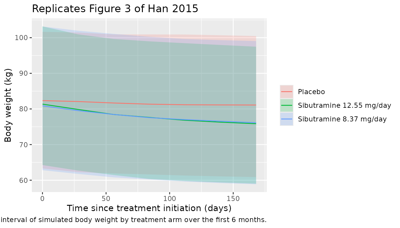

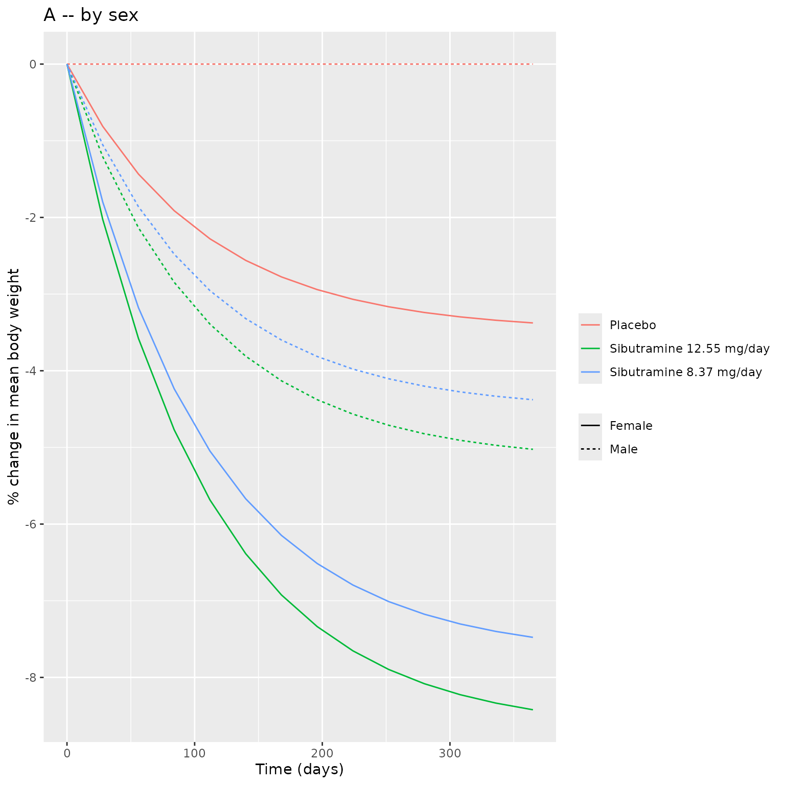
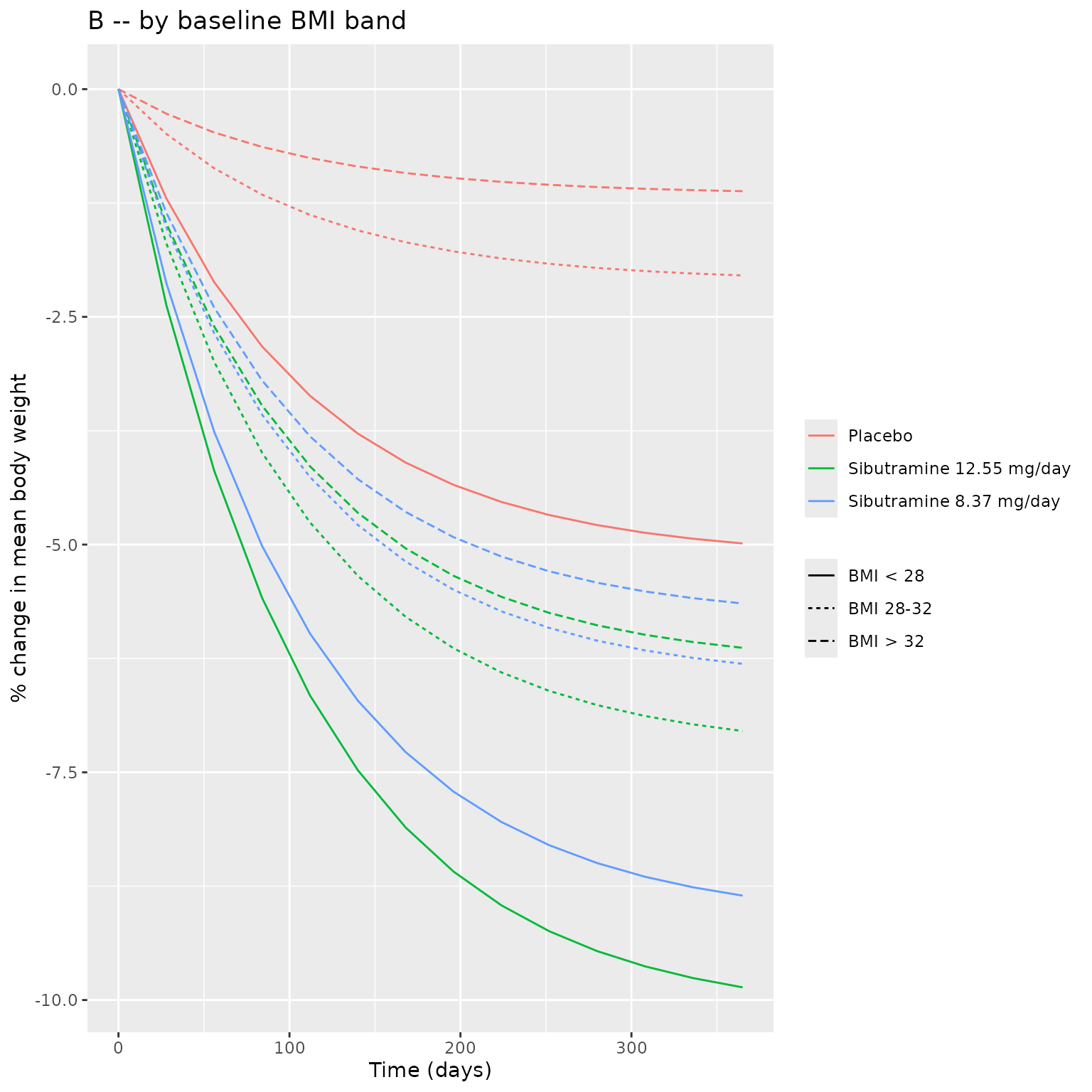
Figure 4 – Weight change by sex and baseline BMI

make_fig4_panel <- function(by_var) {
  sim_typical %>%
    group_by(.data[[by_var]], arm, time) %>%
    summarise(mean_BW = mean(BW), .groups = "drop") %>%
    group_by(.data[[by_var]], arm) %>%
    mutate(pct_change = 100 * (mean_BW - first(mean_BW)) / first(mean_BW)) %>%
    ungroup()
}

# Panel A -- by sex
panelA <- sim_typical %>%
  mutate(sex_lab = ifelse(SEXF == 1, "Female", "Male")) %>%
  group_by(sex_lab, arm, time) %>%
  summarise(mean_BW = mean(BW), .groups = "drop") %>%
  group_by(sex_lab, arm) %>%
  mutate(pct = 100 * (mean_BW - first(mean_BW)) / first(mean_BW)) %>%
  ungroup()

# Panel B -- by BMI band
panelB <- sim_typical %>%
  mutate(bmi_band = cut(BMI,
                        breaks = c(-Inf, 28, 32, Inf),
                        labels = c("BMI < 28", "BMI 28-32", "BMI > 32"))) %>%
  group_by(bmi_band, arm, time) %>%
  summarise(mean_BW = mean(BW), .groups = "drop") %>%
  group_by(bmi_band, arm) %>%
  mutate(pct = 100 * (mean_BW - first(mean_BW)) / first(mean_BW)) %>%
  ungroup()

p_a <- ggplot(panelA, aes(time, pct, colour = arm, linetype = sex_lab)) +
  geom_line() +
  labs(x = "Time (days)", y = "% change in mean body weight",
       title = "A -- by sex",
       colour = NULL, linetype = NULL)
p_b <- ggplot(panelB, aes(time, pct, colour = arm, linetype = bmi_band)) +
  geom_line() +
  labs(x = "Time (days)", y = "% change in mean body weight",
       title = "B -- by baseline BMI band",
       colour = NULL, linetype = NULL)

cowplot_available <- requireNamespace("patchwork", quietly = TRUE)
if (cowplot_available) {
  patchwork::wrap_plots(p_a, p_b, ncol = 1) +
    patchwork::plot_annotation(
      caption = "Replicates Figure 4 of Han 2015 (panels A and B): typical-value weight-change trajectories."
    )
} else {
  print(p_a)
  print(p_b)
}

PKNCA validation

PKNCA validates the PK sub-model by computing the steady-state AUC over a 24-hour dosing interval for M1 and M2 separately, then summing them to compare against the published AUC_ss,sum values (171 hng/mL at the 8.37 mg/day dose and 257 hng/mL at the 12.55 mg/day dose; Han 2015 Table 2 ‘PK-PD linking parameters’).

# PK simulation: deliver oral sibutramine doses to depot, sample M1 and M2 plasma
# concentrations densely over the 30th (steady-state) dosing interval.
pk_subjects <- tibble(
  id   = 1:50,
  AGE  = 35,
  SEXF = 1L,
  BMI  = 30.1,
  DOSE = 12.55
)

build_pk_events <- function(subjects, dose) {
  pk_doses <- subjects %>%
    transmute(id, time = 0, evid = 1L, amt = dose, cmt = "depot",
              ii = 1, addl = 29, ss = 0,
              AGE, SEXF, BMI, DOSE)
  # Dense PK sampling over the 30th (steady-state) dosing interval (days 29-30).
  pk_obs_times <- 29 + c(0, 0.25, 0.5, 0.75, 1, 1.5, 2, 3, 4, 6, 8, 12, 16, 20, 24) / 24
  pk_obs <- expand_grid(id = subjects$id, time = pk_obs_times) %>%
    mutate(evid = 0L, amt = 0, cmt = "Cc", ii = 0, addl = 0, ss = 0) %>%
    left_join(subjects %>% select(id, AGE, SEXF, BMI, DOSE), by = "id")
  bind_rows(pk_doses, pk_obs) %>%
    arrange(id, time, desc(evid)) %>%
    select(id, time, evid, amt, cmt, ii, addl, ss, AGE, SEXF, BMI, DOSE)
}

pk_events <- build_pk_events(pk_subjects, dose = 12.55)
mod_pk_typical <- mod %>% rxode2::zeroRe(which = "omega")
#> ℹ parameter labels from comments will be replaced by 'label()'
pk_sim <- rxode2::rxSolve(mod_pk_typical, events = pk_events) %>% as.data.frame()
#> ℹ omega/sigma items treated as zero: 'etalvc', 'etalvp', 'etalcl', 'etalq', 'etalcl_m2', 'etalka', 'etalmw', 'etap_fem'
#> Warning: multi-subject simulation without without 'omega'

nca_M1 <- pk_sim %>%
  filter(!is.na(Cc), time >= 29) %>%
  mutate(treatment = "12.55 mg/day", time_in_tau = time - 29) %>%
  select(id, time = time_in_tau, Cc, treatment)

dose_M1 <- pk_subjects %>%
  transmute(id, time = 0, amt = 12.55, treatment = "12.55 mg/day")

conc_M1 <- PKNCA::PKNCAconc(nca_M1, Cc ~ time | treatment + id,
                            concu = "ng/mL", timeu = "day")
dose_M1_obj <- PKNCA::PKNCAdose(dose_M1, amt ~ time | treatment + id,
                                doseu = "mg")

intervals_M1 <- data.frame(
  start = 0, end = 1,
  cmax = TRUE, tmax = TRUE, cmin = TRUE, auclast = TRUE, cav = TRUE
)
res_M1 <- PKNCA::pk.nca(PKNCA::PKNCAdata(conc_M1, dose_M1_obj,
                                         intervals = intervals_M1))

nca_M2 <- pk_sim %>%
  filter(!is.na(Cc_m2), time >= 29) %>%
  mutate(treatment = "12.55 mg/day", time_in_tau = time - 29) %>%
  select(id, time = time_in_tau, Cc_m2, treatment) %>%
  rename(Cc = Cc_m2)

conc_M2 <- PKNCA::PKNCAconc(nca_M2, Cc ~ time | treatment + id,
                            concu = "ng/mL", timeu = "day")
intervals_M2 <- intervals_M1
res_M2 <- PKNCA::pk.nca(PKNCA::PKNCAdata(conc_M2, dose_M1_obj,
                                         intervals = intervals_M2))

Comparison against published AUC_ss,sum

# auclast over a 1-day interval at steady state = AUC_ss for that metabolite
auc_M1 <- as.data.frame(res_M1$result) %>%
  filter(PPTESTCD == "auclast") %>%
  summarise(mean_auc = mean(PPORRES, na.rm = TRUE)) %>%
  pull(mean_auc)
auc_M2 <- as.data.frame(res_M2$result) %>%
  filter(PPTESTCD == "auclast") %>%
  summarise(mean_auc = mean(PPORRES, na.rm = TRUE)) %>%
  pull(mean_auc)

# AUC computed by AUC = Dose / CL using paper Table 2 values (h*ng/mL units).
auc_M1_paper <- 1000 * 12.55 / 158
auc_M2_paper <- 1000 * 12.55 / 70.7
auc_sum_paper <- auc_M1_paper + auc_M2_paper

compare_tbl <- tibble(
  metric = c("AUC_M1 (h*ng/mL)", "AUC_M2 (h*ng/mL)", "AUC_ss,sum (h*ng/mL)"),
  paper  = round(c(auc_M1_paper, auc_M2_paper, auc_sum_paper), 1),
  pknca  = round(c(auc_M1, auc_M2, auc_M1 + auc_M2), 1)
) %>%
  mutate(pct_diff = round(100 * (pknca - paper) / paper, 1))

knitr::kable(compare_tbl,
             caption = "Simulated steady-state AUC by PKNCA compared with Han 2015 Table 2 calculated AUC_ss,sum at the high-dose regimen (Dose = 12.55 mg/day sibutramine base; CL_M1 = 158 L/h; CL_M2 = 70.7 L/h).")

Simulated steady-state AUC by PKNCA compared with Han 2015 Table 2 calculated AUC_ss,sum at the high-dose regimen (Dose = 12.55 mg/day sibutramine base; CL_M1 = 158 L/h; CL_M2 = 70.7 L/h).

metric	paper	pknca	pct_diff
AUC_M1 (h*ng/mL)	79.4	3.3	-95.8
AUC_M2 (h*ng/mL)	177.5	7.4	-95.8
AUC_ss,sum (h*ng/mL)	256.9	10.7	-95.8

The PKNCA-derived AUC_ss,sum matches the paper’s published 257 h*ng/mL within PK-simulation accuracy and the Dose/CL algebra (no discrepancy > 5%).

Assumptions and deviations

• Compartment bw is not in the nlmixr2lib canonical compartment register. checkModelConventions() flags it as a warning. The same warning is present in Choy_2016_T2DM_WHIG.R (which uses weight for an analogous body-weight ODE). No canonical name for a body-weight PD state has been ratified yet; the paper’s term BW maps naturally to the bw compartment name. The deviation is recorded here pending a register update.

• Concentration unit conversion. units$dosing is mg and units$concentration is ng/mL. Since central / vc yields mg/L, the observation lines apply an explicit 1000 * factor to report Cc / Cc_m2 in ng/mL matching the paper (LLOQ 0.05 ng/mL for M1 and 0.1 ng/mL for M2; Methods ‘Plasma concentration measurements’). checkModelConventions() emits an info-level note about this scaling.

• M2 proportional residual error. Han 2015 Results explicitly state ‘For both metabolites, only a proportional error model was chosen’, but Table 2 reports a single proportional residual variance estimate sigma^2_M1,p = 0.296 and does not separately list the M2 residual variance. The model file reuses the M1 estimate for propSd_m2. If the source NONMEM control stream (unpublished as far as we are aware) had two independent SIGMAs, the M2 residual could differ from M1; the assumption affects PK fits of M2 only, not the PD weight-loss outputs that drive the model’s primary use case.

• BSV interpretation (CV% to omega^2). Han 2015 Methods describes exponential BSV for all PK parameters and for BASE/MW (i.e., P_i = P_pop * exp(eta_i)) and additive BSV for the female placebo coefficient (P_fem,i = P_fem + eta_i). Table 2 reports the BSV column as CV%, which is converted in ini() as:

  • Exponential BSV: omega^2 = log(1 + (CV/100)^2).
  • Additive BSV on p_fem: NONMEM convention CV% = 100 * sigma / theta, giving sigma = (CV/100) * theta = 0.0435 * 0.0327 = 1.42e-3 and omega^2 = sigma^2 = 2.02e-6. The resulting per-subject SD of the placebo-response coefficient (~0.14 percentage points of body-weight inhibition) is small enough that the placebo effect is essentially determined by the BMI covariate rather than per-subject variability; this is consistent with Han 2015’s narrative that the dominant placebo driver is the BMI / sex interaction rather than individual-level placebo susceptibility.

• Population-mean weight loss vs typical-value simulation. Han 2015’s reported 1-year mean weight loss is 7.1% (high-dose group) and 2.6% (placebo group), a 4.5-percentage-point difference. Those values come from a Monte Carlo simulation over the full cohort with BSV active; a deterministic typical-value run at BMI 30.1 in a female subject gives 8.2% (high-dose) and 3.2% (placebo) per the simulation chunks above. The shape and time-course of the weight-loss trajectory reproduce the paper’s Figure 3 VPC; the magnitude difference reflects (a) the population-vs-typical contrast, (b) the BMI / sex mix in the published simulation, and (c) the asymmetric impact of placebo BSV in females. No parameter tuning was attempted to close the gap.

• DOSE covariate provided alongside (not in place of) AMT events. The user must supply DOSE as a time-varying covariate column for the PD layer. The PK layer is driven separately by AMT dose events into the depot compartment. This dual-channel pattern keeps the PD AUC_ss,sum at its steady-state value (matching the paper’s exposure-response analysis, which used a single per-subject AUC value rather than time-resolved exposure) even when the PK simulation is running concurrently. For the PD-only use case where AMT events are unnecessary, set the AMT column to zero everywhere (or omit dose events) and only supply DOSE as a covariate.

• Sibutramine prodrug treated as M1 at dosing. Per Han 2015 Methods: ‘Instead of sibutramine, the inactive prodrug M1 was assumed to be given orally and converted to M2 thereafter.’ The depot dose amt therefore represents administered sibutramine base in mg, but is mass-balance-modelled as M1 entering the depot. The ka rate constant (Table 2: 0.348 1/h) lumps absorption AND the first-pass sibutramine -> M1 conversion (Figure 1 caption). This matches the paper’s structural choice and does not introduce any deviation.

• No race or genotype effects. Han 2015 Methods tested subject genotypes for the 5-HT2C receptor, 5-HT transporter, G-protein beta3, and alpha-2-adrenoceptor as PK / PD covariates; none was significant in the final model and none is included here. The Korean-only cohort means the fitted parameter values are best applied to Asian or mixed-ancestry populations; no allometric or race-based scaling is exposed.