Olmesartan + amlodipine + hydrochlorothiazide fixed-dose combination CS-8635 (Song 2013)
Source:vignettes/articles/Song_2013_olmesartan_amlodipine_hydrochlorothiazide.Rmd
Song_2013_olmesartan_amlodipine_hydrochlorothiazide.RmdModels and source
Song 2013 built five models: a population PK model for each of the three CS-8635 components, and two exposure-response (E-R) models – one for diastolic and one for systolic seated trough blood pressure. All five are packaged separately, as the authors fitted them.
modellib() name |
Role | Source table |
|---|---|---|
Song_2013_olmesartan |
2-compartment popPK, olmesartan | Table S3, Eq. 8 |
Song_2013_amlodipine |
2-compartment popPK, amlodipine | Table S4, Eq. 9 |
Song_2013_hydrochlorothiazide |
2-compartment popPK, hydrochlorothiazide | Table S5, Eq. 10 |
Song_2013_olmesartan_amlodipine_hydrochlorothiazide_dbp |
E-R, change from baseline in SeDBP | Table S6, Eq. 1-7 |
Song_2013_olmesartan_amlodipine_hydrochlorothiazide_sbp |
E-R, change from baseline in SeSBP | Table S7, Eq. 1-7 |
- Citation: Song S, Carrothers TJ, Moore H, Green M, Miller R, Rohatagi S, Lee J, Wang A, Melino M, Patel M, Heyrman R, Salazar DE. Model-supported development of CS-8635: a fixed-dose combination of olmesartan, amlodipine, and hydrochlorothiazide. Clin Pharmacol Drug Dev. 2013;2(2):103-112. doi:10.1002/cpdd.17. Structural parameters and inter-subject variability from Supplemental Table S3; the clearance covariate model from main-text Equation 8.
- Article: https://doi.org/10.1002/cpdd.17
The three PK models and the two E-R models are joined by a single scalar per drug per subject. Song 2013’s M&S Methods define it explicitly:
… BP lowering effects of these compounds could be successfully linked to steady-state exposures, represented by area-under-the-curve (AUCss), calculated as Dose divided by Apparent Clearance.
So AUC_OLM, AUC_AML and
AUC_HCTZ are Dose / (CL/F), and the PK models
exist in this library chiefly to generate them. That identity is the
first thing this vignette checks.
Population
The pooled exposure-response dataset is 4873 adults with hypertension from three placebo-controlled factorial phase III trials (Song 2013 Table 2): 866-318 (n = 495, olmesartan + hydrochlorothiazide), CS8663-A-U301 / COACH (n = 1920, olmesartan + amlodipine) and CS8635-A-U301 / TRINITY (n = 2458, the triple combination). Mean baseline seated trough blood pressure was 165/102 mmHg, mean age 54.8 (SD 11) years, mean weight 94.9 (SD 22) kg, 46.1% female, and the race/ethnicity split was 58.9% White / 25.0% Black / 13.4% Hispanic / 1.9% Asian / 0.8% Other. 14.1% were diabetic.
Pharmacokinetic data were available for only 1471 of those subjects. The population PK models therefore pool the sparse phase III sampling with 13 phase I clinical-pharmacology studies that had full-profile sampling (Song 2013 Table S1), giving n = 1927 for olmesartan and amlodipine and n = 1278 for hydrochlorothiazide – the hydrochlorothiazide dataset excludes CS8663-A-U301, whose program studied olmesartan + amlodipine only.
The same information is available programmatically from each model’s
population metadata, e.g.
readModelDb("Song_2013_olmesartan_amlodipine_hydrochlorothiazide_dbp")()$population.
Source trace
The per-parameter origin is recorded as an in-file comment next to
each ini() entry. The table below collects the structural
provenance in one place.
| Equation / parameter | Value | Source location |
|---|---|---|
Response = Placebo + Drug Effect |
n/a | Song 2013 Eq. 1, p. 105 |
Drug Effect = MonoOM + MonoAML + MonoHCTZ + Interaction |
n/a | Song 2013 Eq. 2, p. 105 |
| Interaction (3 pairwise + 1 three-way product terms) | n/a | Song 2013 Eq. 3, p. 105 |
| Linear drug effect (hydrochlorothiazide) | n/a | Song 2013 Eq. 4, p. 106 |
| Saturable drug effect (olmesartan, amlodipine) | n/a | Song 2013 Eq. 5, p. 106 |
| Continuous covariate form, median-normalized power | n/a | Song 2013 Eq. 6, p. 106 |
Categorical covariate form,
(1 + coefficient * cov)
|
n/a | Song 2013 Eq. 7, p. 106 |
Olmesartan (CL/F) = 6.32 * (CLCR / 111)^0.425
|
6.32 L/h, 0.425 | Song 2013 Eq. 8, p. 107; Table S3 |
Amlodipine (CL/F) = 23.4 * (AGE / 50.9)^-0.349
|
23.4 L/h, -0.349 | Song 2013 Eq. 9, p. 107; Table S4 |
Hydrochlorothiazide
(CL/F) = 20.3 * e^(-0.219*Female) * (CLCR/117.5)^0.499 * (AGE/49.5)^-0.214
|
20.3 L/h | Song 2013 Eq. 10, p. 107; Table S5 |
Olmesartan Vc/F, Vp/F, Q/F,
Ka, ALAG1, IIV, sigmas |
36.8 L, 29.0 L, 1.64 L/h, 1.25 /h, 0.406 h | Song 2013 Table S3 |
Amlodipine Vc/F, Vp/F, Q/F,
Ka, ALAG1, IIV, sigmas |
1060 L, 465 L, 26.6 L/h, 0.215 /h, 0.315 h | Song 2013 Table S4 |
Hydrochlorothiazide V2, V3,
Q/F, Ka, ALAG1, IIV, sigmas |
27.7 L, 174 L, 18.3 L/h, 0.364 /h, 0.419 h | Song 2013 Table S5 |
| Diastolic E-R: every placebo, Emax, EAUC50, slope, covariate and interaction estimate | see model file | Song 2013 Table S6 |
| Systolic E-R: every placebo, Emax, EAUC50, slope, covariate and interaction estimate | see model file | Song 2013 Table S7 |
| Diastolic / systolic additive IIV | 8.56 / 14.0 mmHg | Song 2013 Tables S6, S7 footnote b (square root of the ETA estimate) |
| Diastolic / systolic residual error | 3.62 / 6.02 mmHg | Song 2013 Tables S6, S7 footnote d (square root of EPS) |
| Answer key: observed and predicted BP lowering by dose | see below | Song 2013 Table 4 |
| Cohort demographics | see below | Song 2013 Tables 2 and S1 |
Two rows of main-text Table 3 carry the right numbers under the wrong labels; the Supplemental tables and narrative are used instead. See Assumptions and deviations below.
Part 1 – Population PK and the AUCss identity
Virtual cohort
The PK cohort reproduces the CS8635-A-U301 phase III PK subset (Song 2013 Table S1: n = 956, age 55.8 (SD 10) years, weight 95.5 (SD 22) kg, CLCR 117 (SD 43) mL/min, 439/956 female). Covariates are drawn with base R’s RNG so the cohort is byte-identical on any rxode2 build.
set.seed(20130217)
n_pk <- 100

pk_cov <- tibble(
  id   = seq_len(n_pk),
  AGE  = pmax(18, rnorm(n_pk, 55.8, 10)),
  WT   = pmax(40, rnorm(n_pk, 95.5, 22)),
  CRCL = pmax(20, rnorm(n_pk, 117, 43)),
  SEXF = rbinom(n_pk, 1, 439 / 956)
)

# Highest marketed CS-8635 strength: olmesartan 40 / amlodipine 10 /
# hydrochlorothiazide 25 mg once daily -- the only strength TRINITY tested.
pk_drugs <- tibble(
  drug  = c("Olmesartan 40 mg", "Amlodipine 10 mg", "Hydrochlorothiazide 25 mg"),
  model = c("Song_2013_olmesartan", "Song_2013_amlodipine",
            "Song_2013_hydrochlorothiazide"),
  amt   = c(40, 10, 25)
)

# Once daily to steady state, then a dense profile over the final dosing
# interval. The grid is fine early (0.05 h) because olmesartan's absorption is
# fast, and coarser over the elimination phase where trapezoids are accurate.
n_dose  <- 60L
t_last  <- 24 * (n_dose - 1L)
obs_grid <- sort(unique(c(
  seq(t_last, t_last + 6, by = 0.05),
  seq(t_last + 6, t_last + 24, by = 0.25)
)))

make_pk_events <- function(dose_mg) {
  bind_rows(
    pk_cov |> mutate(time = 0, amt = dose_mg, evid = 1L, ii = 24,
                     addl = n_dose - 1L, cmt = "depot"),
    tidyr::expand_grid(pk_cov, time = obs_grid) |>
      mutate(amt = NA_real_, evid = 0L, ii = 0, addl = 0L, cmt = "central")
  ) |>
    arrange(id, time, desc(evid))
}
# zeroRe() strips the omega matrix, so rxode2 warns once per solve that a
# multi-subject simulation has no 'omega'. That is precisely the intent here --
# every assertion in this vignette runs on deterministic typical-value solves
# over a base-R-seeded covariate cohort, so nothing depends on which rxode2
# build draws which random effect. The message is muffled by name rather than
# with a blanket suppressWarnings(), so any other warning still surfaces.
solve_typical <- function(mod, ev) {
  withCallingHandlers(
    rxode2::rxSolve(mod, as.data.frame(ev), returnType = "data.frame"),
    warning = function(w) {
      if (grepl("omega", conditionMessage(w), fixed = TRUE)) {
        invokeRestart("muffleWarning")
      }
    }
  )
}
Simulation
Two solves per drug. The typical-value solve (zeroRe())
is the one every assertion below uses: it is fully deterministic given
the seeded covariate cohort, so nothing here depends on which rxode2
build draws which random effect. The IIV solve is used only for the
visual predictive check.
pk_sim <- lapply(seq_len(nrow(pk_drugs)), function(i) {
  mod <- rxode2::rxode2(readModelDb(pk_drugs$model[i]))
  ev  <- make_pk_events(pk_drugs$amt[i])
  list(
    drug    = pk_drugs$drug[i],
    typical = solve_typical(rxode2::zeroRe(mod), ev) |>
      mutate(drug = pk_drugs$drug[i]),
    iiv     = rxode2::rxSolve(mod, ev, returnType = "data.frame") |>
      mutate(drug = pk_drugs$drug[i])
  )
})
#> ℹ parameter labels from comments will be replaced by 'label()'
#> ℹ omega/sigma items treated as zero: 'etalcl', 'etalvc', 'etalvp', 'etalq', 'etalka'
#> ℹ parameter labels from comments will be replaced by 'label()'
#> ℹ omega/sigma items treated as zero: 'etalcl', 'etalvc', 'etalvp', 'etalka'
#> ℹ parameter labels from comments will be replaced by 'label()'
#> ℹ omega/sigma items treated as zero: 'etalcl', 'etalvc', 'etalvp', 'etalq', 'etalka'
names(pk_sim) <- pk_drugs$drug

pk_typ <- bind_rows(lapply(pk_sim, `[[`, "typical"))
pk_iiv <- bind_rows(lapply(pk_sim, `[[`, "iiv"))
Replicate Figure 1
Song 2013 Figure 1 is a post-predictive check of each component’s plasma concentration over the 0-30 h window after a dose at steady state in CS8635-A-U301, with the mean and the 2.5th / 97.5th percentiles of the simulation drawn as solid and dotted lines. The panel below is the same quantity from the packaged models, plotted against time since the last dose.
# Replicates Figure 1 of Song 2013: mean and 2.5 / 97.5 percentile prediction
# interval of the plasma concentration at steady state, one panel per drug.
pk_iiv |>
  filter(time >= t_last) |>
  mutate(tad = time - t_last) |>
  group_by(drug, tad) |>
  summarise(Mean = mean(Cc), Q025 = quantile(Cc, 0.025),
            Q975 = quantile(Cc, 0.975), .groups = "drop") |>
  mutate(drug = factor(drug, levels = pk_drugs$drug)) |>
  ggplot(aes(tad)) +
  geom_ribbon(aes(ymin = Q025, ymax = Q975), alpha = 0.2) +
  geom_line(aes(y = Q025), linetype = "dotted") +
  geom_line(aes(y = Q975), linetype = "dotted") +
  geom_line(aes(y = Mean), linewidth = 0.8) +
  facet_wrap(~drug, ncol = 1, scales = "free_y") +
  labs(x = "Time after dose at steady state (h)",
       y = "Plasma concentration (ng/mL)",
       caption = "Replicates Figure 1 of Song 2013.")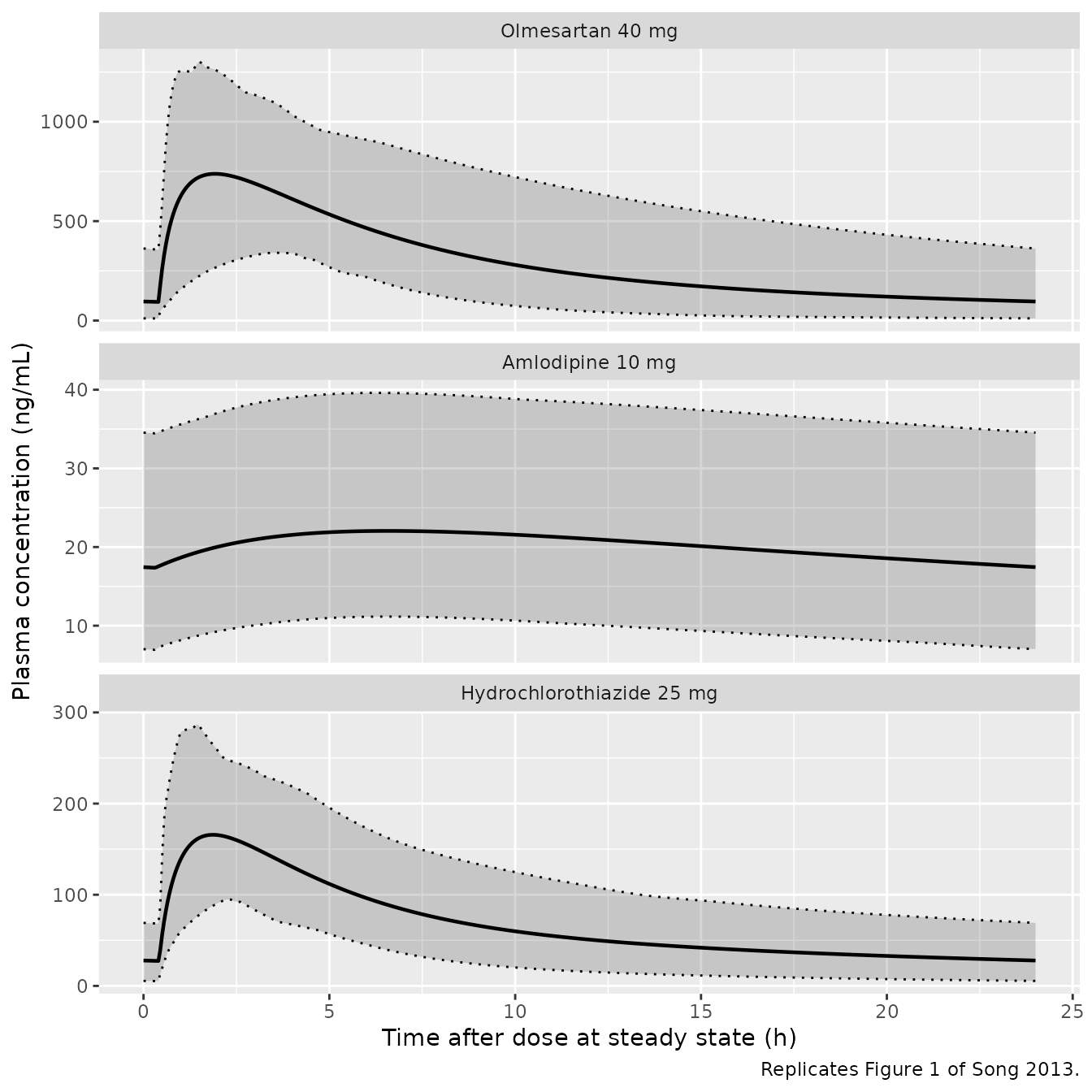
PKNCA validation of the AUCss identity
The exposure-response models consume Dose / (CL/F). This
section computes the steady-state AUC over the final dosing interval
with PKNCA and checks it against that closed form, per subject. Both
sides use the same individual clearance, so the only difference is
trapezoidal error and the assertion can be tight.
nca_conc <- pk_typ |>
  filter(!is.na(Cc), time >= t_last) |>
  mutate(time = time - t_last) |>
  select(id, time, Cc, drug)

# Guarantee a time-zero row per (id, drug). At steady state the pre-dose
# concentration is the trough carried over from the previous interval, which
# the grid above already supplies at time == t_last, so this only fires
# defensively.
nca_conc <- bind_rows(
  nca_conc,
  nca_conc |> distinct(id, drug) |> mutate(time = 0, Cc = 0)
) |>
  distinct(id, drug, time, .keep_all = TRUE) |>
  arrange(id, drug, time)

conc_obj <- PKNCA::PKNCAconc(as.data.frame(nca_conc), Cc ~ time | drug + id)

nca_dose <- pk_drugs |>
  select(drug, amt) |>
  tidyr::expand_grid(id = pk_cov$id) |>
  mutate(time = 0) |>
  as.data.frame()

dose_obj <- PKNCA::PKNCAdose(nca_dose, amt ~ time | drug + id)

intervals <- data.frame(start = 0, end = 24,
                        cmax = TRUE, tmax = TRUE, auclast = TRUE)

nca_res <- PKNCA::pk.nca(
  PKNCA::PKNCAdata(conc_obj, dose_obj, intervals = intervals)
)
# Closed form: AUCss = Dose / (CL/F), with the individual CL/F rebuilt from the
# packaged covariate models (Song 2013 Eq. 8, 9 and 10).
closed_form <- bind_rows(
  pk_cov |> mutate(drug = "Olmesartan 40 mg",
                   cl = 6.32 * (CRCL / 111)^0.425, amt = 40),
  pk_cov |> mutate(drug = "Amlodipine 10 mg",
                   cl = 23.4 * (AGE / 50.9)^-0.349, amt = 10),
  pk_cov |> mutate(drug = "Hydrochlorothiazide 25 mg",
                   cl = 20.3 * exp(-0.219 * SEXF) *
                     (CRCL / 117.5)^0.499 * (AGE / 49.5)^-0.214, amt = 25)
) |>
  mutate(auc_closed = amt / cl * 1000) |>   # mg / (L/h) -> ng*h/mL
  select(id, drug, auc_closed)

auc_chk <- as.data.frame(nca_res) |>
  filter(PPTESTCD == "auclast") |>
  select(id, drug, auc_nca = PPORRES) |>
  inner_join(closed_form, by = c("id", "drug")) |>
  mutate(pct_diff = 100 * (auc_nca - auc_closed) / auc_closed)

auc_chk |>
  group_by(drug) |>
  summarise(n = n(),
            `Median AUCss, PKNCA (ng*h/mL)` = median(auc_nca),
            `Median AUCss, Dose/(CL/F) (ng*h/mL)` = median(auc_closed),
            `Max |% difference|` = max(abs(pct_diff)), .groups = "drop") |>
  rename(Drug = drug, N = n) |>
  knitr::kable(digits = c(0, 0, 1, 1, 3),
               caption = paste("Steady-state AUC from PKNCA against the",
"paper's own closed form, Dose / (CL/F)."))| Drug | N | Median AUCss, PKNCA (ng*h/mL) | Median AUCss, Dose/(CL/F) (ng*h/mL) | Max |% difference| |
|---|---|---|---|---|
| Amlodipine 10 mg | 100 | 440.4 | 440.4 | 0.001 |
| Hydrochlorothiazide 25 mg | 100 | 1393.2 | 1393.2 | 0.007 |
| Olmesartan 40 mg | 100 | 6257.7 | 6257.7 | 0.001 |
# A solve against its own closed form: the residual is pure trapezoidal error
# on a common set of drawn parameters, so a tight all() bound is correct here.
stopifnot(all(abs(auc_chk$pct_diff) < 0.5))
The identity holds to well under 1% for every subject and every component, so the packaged PK models deliver exactly the exposure metric the exposure-response models were built on.
nca_summary <- as.data.frame(nca_res) |>
  filter(PPTESTCD %in% c("cmax", "tmax", "auclast")) |>
  group_by(drug, PPTESTCD) |>
  summarise(value = median(PPORRES), .groups = "drop") |>
  tidyr::pivot_wider(names_from = PPTESTCD, values_from = value) |>
  mutate(drug = factor(drug, levels = pk_drugs$drug)) |>
  arrange(drug)

nca_summary |>
  rename("Drug" = drug, "Cmax (ng/mL)" = cmax, "Tmax (h)" = tmax,
         "AUC0-24,ss (ng*h/mL)" = auclast) |>
  knitr::kable(digits = 1,
               caption = paste("Median simulated steady-state NCA for the",
                               "TRINITY high-dose strength (40/10/25 mg).",
                               "Song 2013 reports no NCA table, so these are",
"presented for orientation only."))| Drug | AUC0-24,ss (ng*h/mL) | Cmax (ng/mL) | Tmax (h) |
|---|---|---|---|
| Olmesartan 40 mg | 6257.7 | 782.1 | 2.1 |
| Amlodipine 10 mg | 440.4 | 20.0 | 7.0 |
| Hydrochlorothiazide 25 mg | 1393.2 | 171.0 | 1.9 |
Part 2 – Exposure-response
Structure
Each E-R model assembles the change from baseline in seated trough blood pressure as
Response = Placebo(study, baseline BP, age, race)
         + MonoOM   (saturable in AUC_OLM)
         + MonoAML  (saturable in AUC_AML)
         + MonoHCTZ (linear in AUC_HCTZ)
         + Interaction(products of the three mono terms)
The monotherapy terms are negative (blood-pressure lowering), so a positive pairwise interaction coefficient acting on the product of two negatives makes the pair sub-additive – Song 2013’s observation that combination effects are “roughly additive, with patients seeing less than 100% of the sum benefit”. The three-way term acts on a product of three negatives and adds a little lowering back.
Virtual cohort
The cohort reproduces the CS8635-A-U301 study population (Song 2013
Table 2: n = 2458, baseline 169/101 mmHg, age 55.2 (SD 11) years, weight
96.1 (SD 23) kg, 1154/2458 female, 704/2458 Black, 365/2458 Hispanic),
because Song 2013 Table 4’s right-hand “Predicted” column is explicitly
“Model predicted BP lowering effects in the CS8635-A-U301 study”. As in
Part 1, covariates come from base R’s RNG and the models are solved with
zeroRe(), so the whole comparison is deterministic.
set.seed(20130217)
n_er <- 200

er_cov <- tibble(
  id            = seq_len(n_er),
  time          = 0,
  evid          = 0L,
  SBP           = rnorm(n_er, 169, 14),
  DBP           = rnorm(n_er, 101, 7.8),
  AGE           = pmax(20, rnorm(n_er, 55.2, 11)),
  WT            = pmax(40, rnorm(n_er, 96.1, 23)),
  SEXF          = rbinom(n_er, 1, 1154 / 2458),
  RACE_BLACK    = rbinom(n_er, 1, 704 / 2458),
  RACE_HISPANIC = rbinom(n_er, 1, 365 / 2458),
  STUDY_CS8635_A_U301 = 1,
  STUDY_CS8663_A_U301 = 0,
  STUDY_866_318       = 0
)

# Typical clearances from Song 2013 Eq. 8-10 at their own centering values;
# AUCss = Dose / (CL/F), converted from mg/(L/h) to ng*h/mL.
auc_of <- function(dose_mg, cl_typ) dose_mg / cl_typ * 1000
Simulation and reproduction of Table 4
dbp_mod <- rxode2::zeroRe(rxode2::rxode2(
  readModelDb("Song_2013_olmesartan_amlodipine_hydrochlorothiazide_dbp")))
#> ℹ parameter labels from comments will be replaced by 'label()'
sbp_mod <- rxode2::zeroRe(rxode2::rxode2(
  readModelDb("Song_2013_olmesartan_amlodipine_hydrochlorothiazide_sbp")))
#> ℹ parameter labels from comments will be replaced by 'label()'

er_arm_mean <- function(mod, om_mg, aml_mg, hctz_mg, outcome) {
  ev <- er_cov |>
    mutate(AUC_OLM  = auc_of(om_mg,   6.32),
           AUC_AML  = auc_of(aml_mg, 23.4),
           AUC_HCTZ = auc_of(hctz_mg, 20.3))
  mean(solve_typical(mod, ev)[[outcome]])
}

# Song 2013 Table 4, right-hand "Predicted" column ("Model predicted BP
# lowering effects in the CS8635-A-U301 study"), plus the observed means for
# the four arms that were actually run.
table4 <- tibble::tribble(
  ~arm,                      ~om, ~aml, ~hctz, ~pred_dbp, ~pred_sbp, ~obs_dbp, ~obs_sbp,
  "Placebo",                   0,    0,   0.0,      -4.0,      -4.7,       NA,       NA,
  "OM/AML 20/5",              20,    5,   0.0,     -15.0,     -26.5,       NA,       NA,
  "OM/AML 40/5",              40,    5,   0.0,     -16.0,     -28.2,       NA,       NA,
  "OM/AML 40/10",             40,   10,   0.0,     -18.2,     -32.0,    -17.8,    -31.1,
  "OM/HCTZ 20/12.5",          20,    0,  12.5,     -12.7,     -22.4,       NA,       NA,
  "OM/HCTZ 40/12.5",          40,    0,  12.5,     -14.1,     -24.4,       NA,       NA,
  "OM/HCTZ 40/25",            40,    0,  25.0,     -16.6,     -29.9,    -16.5,    -31.2,
  "CS-8635 20/5/12.5",        20,    5,  12.5,     -16.8,     -30.4,       NA,       NA,
  "CS-8635 40/5/12.5",        40,    5,  12.5,     -17.9,     -32.1,       NA,       NA,
  "CS-8635 40/10/12.5",       40,   10,  12.5,     -19.8,     -35.2,       NA,       NA,
  "CS-8635 40/5/25",          40,    5,  25.0,     -19.8,     -35.9,       NA,       NA
)

table4_sim <- table4 |>
  rowwise() |>
  mutate(sim_dbp = er_arm_mean(dbp_mod, om, aml, hctz, "ddbp"),
         sim_sbp = er_arm_mean(sbp_mod, om, aml, hctz, "dsbp")) |>
  ungroup() |>
  mutate(pct_dbp = 100 * (sim_dbp - pred_dbp) / pred_dbp,
         pct_sbp = 100 * (sim_sbp - pred_sbp) / pred_sbp)
#> ℹ omega/sigma items treated as zero: 'etaddbp'
#> ℹ omega/sigma items treated as zero: 'etaddbp'
#> ℹ omega/sigma items treated as zero: 'etaddbp'
#> ℹ omega/sigma items treated as zero: 'etaddbp'
#> ℹ omega/sigma items treated as zero: 'etaddbp'
#> ℹ omega/sigma items treated as zero: 'etaddbp'
#> ℹ omega/sigma items treated as zero: 'etaddbp'
#> ℹ omega/sigma items treated as zero: 'etaddbp'
#> ℹ omega/sigma items treated as zero: 'etaddbp'
#> ℹ omega/sigma items treated as zero: 'etaddbp'
#> ℹ omega/sigma items treated as zero: 'etaddbp'
#> ℹ omega/sigma items treated as zero: 'etadsbp'
#> ℹ omega/sigma items treated as zero: 'etadsbp'
#> ℹ omega/sigma items treated as zero: 'etadsbp'
#> ℹ omega/sigma items treated as zero: 'etadsbp'
#> ℹ omega/sigma items treated as zero: 'etadsbp'
#> ℹ omega/sigma items treated as zero: 'etadsbp'
#> ℹ omega/sigma items treated as zero: 'etadsbp'
#> ℹ omega/sigma items treated as zero: 'etadsbp'
#> ℹ omega/sigma items treated as zero: 'etadsbp'
#> ℹ omega/sigma items treated as zero: 'etadsbp'
#> ℹ omega/sigma items treated as zero: 'etadsbp'
table4_sim |>
  select(arm, pred_dbp, sim_dbp, pct_dbp, pred_sbp, sim_sbp, pct_sbp) |>
  rename("Regimen (OM/AML/HCTZ, mg)"     = arm,
         "dSeDBP published (mmHg)"       = pred_dbp,
         "dSeDBP simulated (mmHg)"       = sim_dbp,
         "dSeDBP difference (%)"         = pct_dbp,
         "dSeSBP published (mmHg)"       = pred_sbp,
         "dSeSBP simulated (mmHg)"       = sim_sbp,
         "dSeSBP difference (%)"         = pct_sbp) |>
  knitr::kable(digits = 1, align = c("l", rep("r", 6)),
               caption = paste("Simulated versus published mean blood-pressure",
                               "lowering. Published values are the",
"CS8635-A-U301 column of Song 2013 Table 4."))| Regimen (OM/AML/HCTZ, mg) | dSeDBP published (mmHg) | dSeDBP simulated (mmHg) | dSeDBP difference (%) | dSeSBP published (mmHg) | dSeSBP simulated (mmHg) | dSeSBP difference (%) |
|---|---|---|---|---|---|---|
| Placebo | -4.0 | -3.9 | -2.3 | -4.7 | -4.5 | -4.9 |
| OM/AML 20/5 | -15.0 | -14.7 | -2.0 | -26.5 | -26.1 | -1.7 |
| OM/AML 40/5 | -16.0 | -15.7 | -2.0 | -28.2 | -27.8 | -1.3 |
| OM/AML 40/10 | -18.2 | -17.9 | -1.9 | -32.0 | -31.8 | -0.7 |
| OM/HCTZ 20/12.5 | -12.7 | -12.1 | -4.8 | -22.4 | -21.0 | -6.2 |
| OM/HCTZ 40/12.5 | -14.1 | -13.5 | -4.4 | -24.4 | -23.1 | -5.5 |
| OM/HCTZ 40/25 | -16.6 | -15.5 | -6.5 | -29.9 | -27.7 | -7.5 |
| CS-8635 20/5/12.5 | -16.8 | -16.2 | -3.7 | -30.4 | -29.5 | -3.1 |
| CS-8635 40/5/12.5 | -17.9 | -17.3 | -3.5 | -32.1 | -31.1 | -3.1 |
| CS-8635 40/10/12.5 | -19.8 | -19.2 | -2.9 | -35.2 | -34.5 | -2.0 |
| CS-8635 40/5/25 | -19.8 | -18.9 | -4.8 | -35.9 | -34.4 | -4.2 |
stopifnot(
  # Structural: a mis-transcribed Emax, EAUC50, slope or AUC unit conversion
  # moves whole arms by tens of percent and blows this immediately.
  median(abs(table4_sim$pct_dbp)) < 6,
  median(abs(table4_sim$pct_sbp)) < 6,
  # Envelope: the residual gap is dominated by the unprinted covariate medians
  # (see the deviations section), which bite hardest in the arms whose exponents
  # are largest.
  max(abs(table4_sim$pct_dbp)) < 12,
  max(abs(table4_sim$pct_sbp)) < 12,
  # Every arm lowers blood pressure, and every active arm lowers it more than
  # placebo does.
  all(table4_sim$sim_dbp < 0), all(table4_sim$sim_sbp < 0),
  all(table4_sim$sim_dbp[-1] < table4_sim$sim_dbp[1]),
  all(table4_sim$sim_sbp[-1] < table4_sim$sim_sbp[1])
)
Song 2013 states the expected ordering of the five CS-8635 strengths outright:
The BP lowering effects for both SeSBP and SeDBP among the different CS-8635 dose strengths are predicted to be in the following order: 20/5/12.5 < 40/5/12.5 < (40/10/12.5 ~ 40/5/25) < 40/10/25 (OM/AML/HCTZ).
That is a falsifiable claim about the packaged models, so it is asserted rather than described.
strengths <- tibble::tribble(
  ~arm,                 ~om, ~aml, ~hctz,
  "20/5/12.5",           20,    5,  12.5,
  "40/5/12.5",           40,    5,  12.5,
  "40/10/12.5",          40,   10,  12.5,
  "40/5/25",             40,    5,  25.0,
  "40/10/25",            40,   10,  25.0
) |>
  rowwise() |>
  mutate(dSeDBP = er_arm_mean(dbp_mod, om, aml, hctz, "ddbp"),
         dSeSBP = er_arm_mean(sbp_mod, om, aml, hctz, "dsbp")) |>
  ungroup()
#> ℹ omega/sigma items treated as zero: 'etaddbp'
#> ℹ omega/sigma items treated as zero: 'etaddbp'
#> ℹ omega/sigma items treated as zero: 'etaddbp'
#> ℹ omega/sigma items treated as zero: 'etaddbp'
#> ℹ omega/sigma items treated as zero: 'etaddbp'
#> ℹ omega/sigma items treated as zero: 'etadsbp'
#> ℹ omega/sigma items treated as zero: 'etadsbp'
#> ℹ omega/sigma items treated as zero: 'etadsbp'
#> ℹ omega/sigma items treated as zero: 'etadsbp'
#> ℹ omega/sigma items treated as zero: 'etadsbp'

strengths |>
  select(arm, dSeDBP, dSeSBP) |>
  rename("CS-8635 strength (OM/AML/HCTZ, mg)" = arm,
         "dSeDBP (mmHg)" = dSeDBP, "dSeSBP (mmHg)" = dSeSBP) |>
  knitr::kable(digits = 2,
               caption = paste("Simulated mean BP lowering across all five",
                               "CS-8635 dose strengths, four of which were",
"never studied clinically."))| CS-8635 strength (OM/AML/HCTZ, mg) | dSeDBP (mmHg) | dSeSBP (mmHg) |
|---|---|---|
| 20/5/12.5 | -16.19 | -29.47 |
| 40/5/12.5 | -17.27 | -31.11 |
| 40/10/12.5 | -19.22 | -34.48 |
| 40/5/25 | -18.86 | -34.38 |
| 40/10/25 | -20.58 | -37.20 |
stopifnot(
  # 20/5/12.5 < 40/5/12.5 < (40/10/12.5 ~ 40/5/25) < 40/10/25, on both endpoints.
  strengths$dSeDBP[1] > strengths$dSeDBP[2],
  strengths$dSeDBP[2] > strengths$dSeDBP[3],
  strengths$dSeDBP[2] > strengths$dSeDBP[4],
  strengths$dSeDBP[3] > strengths$dSeDBP[5],
  strengths$dSeDBP[4] > strengths$dSeDBP[5],
  strengths$dSeSBP[1] > strengths$dSeSBP[2],
  strengths$dSeSBP[2] > strengths$dSeSBP[3],
  strengths$dSeSBP[2] > strengths$dSeSBP[4],
  strengths$dSeSBP[3] > strengths$dSeSBP[5],
  strengths$dSeSBP[4] > strengths$dSeSBP[5],
  # The paper writes 40/10/12.5 ~ 40/5/25, i.e. within ~0.5 mmHg of each other.
  abs(strengths$dSeDBP[3] - strengths$dSeDBP[4]) < 0.5,
  abs(strengths$dSeSBP[3] - strengths$dSeSBP[4]) < 1.0
)
The interaction is sub-additive
The paper’s central quantitative claim about the combination is that its effect exceeds any component’s but falls short of their arithmetic sum. Because the interaction terms are the only thing standing between the two, this is a direct check on Eq. 3.
er_arm_mean_dbp <- function(om, aml, hctz) er_arm_mean(dbp_mod, om, aml, hctz, "ddbp")

pbo   <- er_arm_mean_dbp(0, 0, 0)
#> ℹ omega/sigma items treated as zero: 'etaddbp'
mono  <- c(OM   = er_arm_mean_dbp(40, 0, 0) - pbo,
           AML  = er_arm_mean_dbp(0, 10, 0) - pbo,
           HCTZ = er_arm_mean_dbp(0, 0, 25) - pbo)
#> ℹ omega/sigma items treated as zero: 'etaddbp'
#> ℹ omega/sigma items treated as zero: 'etaddbp'
#> ℹ omega/sigma items treated as zero: 'etaddbp'
triple <- er_arm_mean_dbp(40, 10, 25) - pbo
#> ℹ omega/sigma items treated as zero: 'etaddbp'

tibble(
  quantity = c("Olmesartan 40 mg alone", "Amlodipine 10 mg alone",
               "Hydrochlorothiazide 25 mg alone",
               "Arithmetic sum of the three",
               "CS-8635 40/10/25 (with interaction)"),
  dSeDBP   = c(mono, sum(mono), triple)
) |>
  rename("Drug effect on dSeDBP, placebo-corrected" = quantity,
         "mmHg" = dSeDBP) |>
  knitr::kable(digits = 2,
               caption = paste("The triple combination beats every component",
                               "but falls short of their sum (Song 2013",
"Discussion)."))| Drug effect on dSeDBP, placebo-corrected | mmHg |
|---|---|
| Olmesartan 40 mg alone | -7.54 |
| Amlodipine 10 mg alone | -9.74 |
| Hydrochlorothiazide 25 mg alone | -4.06 |
| Arithmetic sum of the three | -21.34 |
| CS-8635 40/10/25 (with interaction) | -16.67 |
Dose-response surface
surface <- tidyr::expand_grid(
  om   = c(0, 20, 40),
  aml  = c(0, 5, 10),
  hctz = c(0, 12.5, 25)
) |>
  rowwise() |>
  mutate(dSeDBP = er_arm_mean(dbp_mod, om, aml, hctz, "ddbp"),
         dSeSBP = er_arm_mean(sbp_mod, om, aml, hctz, "dsbp")) |>
  ungroup()
#> ℹ omega/sigma items treated as zero: 'etaddbp'
#> ℹ omega/sigma items treated as zero: 'etaddbp'
#> ℹ omega/sigma items treated as zero: 'etaddbp'
#> ℹ omega/sigma items treated as zero: 'etaddbp'
#> ℹ omega/sigma items treated as zero: 'etaddbp'
#> ℹ omega/sigma items treated as zero: 'etaddbp'
#> ℹ omega/sigma items treated as zero: 'etaddbp'
#> ℹ omega/sigma items treated as zero: 'etaddbp'
#> ℹ omega/sigma items treated as zero: 'etaddbp'
#> ℹ omega/sigma items treated as zero: 'etaddbp'
#> ℹ omega/sigma items treated as zero: 'etaddbp'
#> ℹ omega/sigma items treated as zero: 'etaddbp'
#> ℹ omega/sigma items treated as zero: 'etaddbp'
#> ℹ omega/sigma items treated as zero: 'etaddbp'
#> ℹ omega/sigma items treated as zero: 'etaddbp'
#> ℹ omega/sigma items treated as zero: 'etaddbp'
#> ℹ omega/sigma items treated as zero: 'etaddbp'
#> ℹ omega/sigma items treated as zero: 'etaddbp'
#> ℹ omega/sigma items treated as zero: 'etaddbp'
#> ℹ omega/sigma items treated as zero: 'etaddbp'
#> ℹ omega/sigma items treated as zero: 'etaddbp'
#> ℹ omega/sigma items treated as zero: 'etaddbp'
#> ℹ omega/sigma items treated as zero: 'etaddbp'
#> ℹ omega/sigma items treated as zero: 'etaddbp'
#> ℹ omega/sigma items treated as zero: 'etaddbp'
#> ℹ omega/sigma items treated as zero: 'etaddbp'
#> ℹ omega/sigma items treated as zero: 'etaddbp'
#> ℹ omega/sigma items treated as zero: 'etadsbp'
#> ℹ omega/sigma items treated as zero: 'etadsbp'
#> ℹ omega/sigma items treated as zero: 'etadsbp'
#> ℹ omega/sigma items treated as zero: 'etadsbp'
#> ℹ omega/sigma items treated as zero: 'etadsbp'
#> ℹ omega/sigma items treated as zero: 'etadsbp'
#> ℹ omega/sigma items treated as zero: 'etadsbp'
#> ℹ omega/sigma items treated as zero: 'etadsbp'
#> ℹ omega/sigma items treated as zero: 'etadsbp'
#> ℹ omega/sigma items treated as zero: 'etadsbp'
#> ℹ omega/sigma items treated as zero: 'etadsbp'
#> ℹ omega/sigma items treated as zero: 'etadsbp'
#> ℹ omega/sigma items treated as zero: 'etadsbp'
#> ℹ omega/sigma items treated as zero: 'etadsbp'
#> ℹ omega/sigma items treated as zero: 'etadsbp'
#> ℹ omega/sigma items treated as zero: 'etadsbp'
#> ℹ omega/sigma items treated as zero: 'etadsbp'
#> ℹ omega/sigma items treated as zero: 'etadsbp'
#> ℹ omega/sigma items treated as zero: 'etadsbp'
#> ℹ omega/sigma items treated as zero: 'etadsbp'
#> ℹ omega/sigma items treated as zero: 'etadsbp'
#> ℹ omega/sigma items treated as zero: 'etadsbp'
#> ℹ omega/sigma items treated as zero: 'etadsbp'
#> ℹ omega/sigma items treated as zero: 'etadsbp'
#> ℹ omega/sigma items treated as zero: 'etadsbp'
#> ℹ omega/sigma items treated as zero: 'etadsbp'
#> ℹ omega/sigma items treated as zero: 'etadsbp'

surface |>
  tidyr::pivot_longer(c(dSeDBP, dSeSBP), names_to = "endpoint",
                      values_to = "change") |>
  ggplot(aes(factor(om), change, colour = factor(aml),
             group = factor(aml))) +
  geom_line() +
  geom_point() +
  facet_grid(endpoint ~ paste("HCTZ", hctz, "mg"), scales = "free_y") +
  labs(x = "Olmesartan dose (mg)", y = "Change from baseline (mmHg)",
       colour = "Amlodipine (mg)",
       caption = paste("Full 3 x 3 x 3 factorial surface Song 2013 used M&S to",
                       "avoid running as 27 clinical arms."))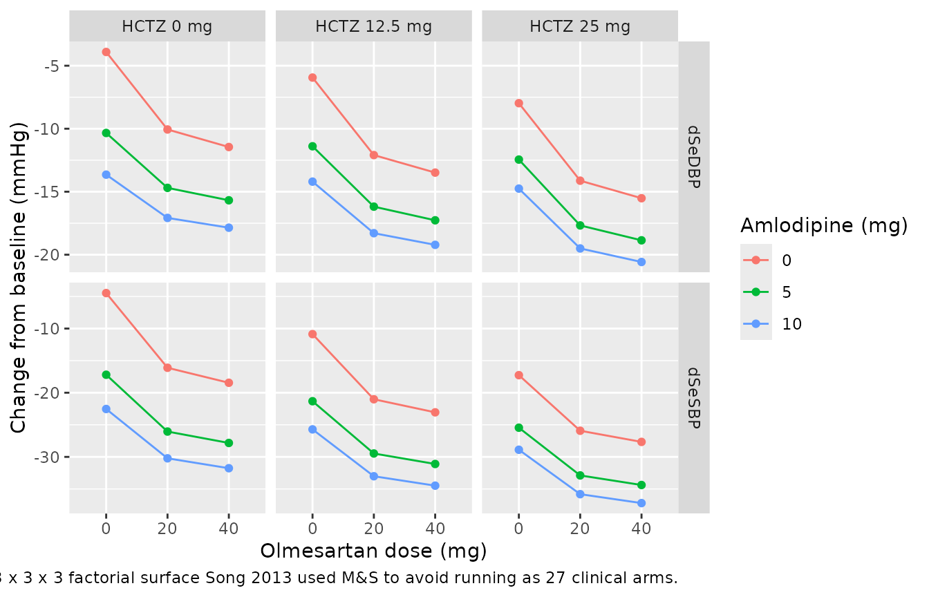
Assumptions and deviations
Unprinted covariate centering values. Song 2013 Eq. 6 normalizes every continuous covariate by “the median observations” of the analysis dataset. The three population PK equations print their own centering values (CLCR 111 and 117.5 mL/min, age 50.9 and 49.5 years), but the body-weight centering value for the volume terms and all four exposure-response centering values are never printed anywhere in the paper or supplement. The packaged models substitute the corresponding dataset means: 91.5 kg (olmesartan / amlodipine PK dataset) and 90.7 kg (hydrochlorothiazide PK dataset), both computed as N-weighted means over Table S1; and baseline SBP 165 mmHg, baseline DBP 102 mmHg, age 54.8 years and weight 94.9 kg for the exposure-response models, from the Table 2 “All data” row. The substitution is calibrated rather than assumed: applying it to the covariates whose medians are printed recovers them to within 1-3% (amlodipine age 50.2 computed vs 50.9 printed; hydrochlorothiazide age 49.3 vs 49.5; olmesartan CLCR 115 vs 111). It is also the dominant source of the residual gap in the Table 4 comparison above, which is systematically in one direction and largest in the arms whose covariate exponents are largest. Body weight on volume does not enter CL/F, so it does not perturb AUCss or anything downstream of it.
Two mislabelled rows in main-text Table 3. The Diastolic column prints -0.818 under “Effect of baseline BP on drug effect of HCTZ”, while Supplemental Table S6 gives the same value as “Effect of age on Drug Effect of OM”. Table S6 is used, for three independent reasons: the Supplemental Results narrative states the diastolic age effect for olmesartan explicitly (“diastolic blood pressure lowering effects might be attenuated in subjects with advanced age”); it confines the hydrochlorothiazide baseline effect to systolic pressure; and a negative baseline exponent on a drug-effect term would contradict the paper’s own repeated finding that higher-baseline subjects show larger treatment effects for all three components. Similarly, the Systolic column’s 0.301 appears in a row labelled only “Sex” grouped under “Placebo effects”, whereas Table S7 labels it “Effect of sex on Drug Effect of AML” and the narrative agrees (“the female subjects might show 30 % higher systolic blood pressure lowering effects of AML”). Both parameters are placed per Tables S6 and S7.
Inconsistent prose percentages for the Black-race effect. Song 2013 Results says “Black subjects showed 39.6% and 29.3% less OM treatment effect on SeDBP and SeSBP”, while the Supplemental Results says “26 and 50 % … for diastolic and systolic”. Both parameter tables agree on -0.263 (diastolic) and -0.393 (systolic), i.e. 26.3% and 39.3%. The tabulated values are used and neither prose sentence is reproducible from them.
Study-specific residual error terms are not encoded. Table S3 reports a third olmesartan sigma, an additive term of 298 (ng/mL)^2 (17.3 ng/mL) applying only to CS8635-A-U301; Table S4 reports the amlodipine equivalent, 1.6 (ng/mL)^2 (1.26 ng/mL); and Table S5 splits the hydrochlorothiazide proportional error by study phase (24.4% phase I, 28.6% phase III). nlmixr2’s error-model syntax cannot switch a residual SD on a covariate, so each model encodes the generally applicable term – proportional plus additive for olmesartan, proportional only for amlodipine, and the phase I proportional value for hydrochlorothiazide – and the study- or phase-specific terms are recorded here and in the model-file comments.
The olmesartan x hydrochlorothiazide interaction is absent from the diastolic model. Table S6 reports it as “n.s.” (Table 3: “NA”). It is carried as
fixed(0)rather than deleted so that the diastolic and systolic files stay structurally identical and the absence is explicit rather than inferred from a missing line.The exposure-response models have no ODE states and no dosing events. Exposure enters only through
AUC_OLM,AUC_AMLandAUC_HCTZ. To remove a component from a regimen, set its AUC column to 0: the corresponding monotherapy term and every interaction term containing it vanish. That is how the mono- and dual-combination arms of Table 4 are simulated above.Cohort covariates are drawn independently. The virtual cohorts sample baseline BP, age, weight, sex and race independently from the marginal distributions of Song 2013 Tables 2 and S1, because no joint distribution or correlation matrix is published. Real correlations (age with renal function, weight with sex) would tighten the simulated spread; they do not shift the arm means the assertions test.
Supplemental Equations S7-S16 are not recoverable from the supplement file. The supplement’s ten exposure-response equations are MathType (
Equation.DSMT4) OLE objects. The.docretains only the field results – itsObjectPoolstorage and the rendered metafile bits are both absent, so the equation images cannot be extracted or rendered. The structure encoded here is therefore taken from main-text Equations 1-7, which are fully legible in the article PDF and which the supplement describes S7-S16 as instantiating. Which parameter each covariate multiplies is pinned independently by the Table S6 / S7 row labels, which name the target explicitly (“Effect of age on Drug Effect of OM”, “Effect of sex on Drug Effect of AML”), and corroborated a third time by the Supplemental Results narrative. Nothing in the packaged models rests on the undecodable images.No parameter value in any of the five models came from outside the paper. Every
ini()entry traces to Song 2013 Tables S3-S7 or main-text Equations 8-10. The centering values discussed in the first bullet are the only quantities computed rather than transcribed, and each is derived from the paper’s own Table S1 or Table 2.