Atorvastatin (Knebel 2013)
Source:vignettes/articles/Knebel_2013_atorvastatin.Rmd
Knebel_2013_atorvastatin.RmdModel and source
#> ℹ parameter labels from comments will be replaced by 'label()'Citation: Knebel W, Gastonguay MR, Malhotra B, El-Tahtawy A, Jen F, Gandelman K. Population pharmacokinetics of atorvastatin and its active metabolites in children and adolescents with heterozygous familial hypercholesterolemia: selective use of informative prior distributions from adults. J Clin Pharmacol. 2013;53(5):505-516. doi:10.1002/jcph.66.
Article: https://doi.org/10.1002/jcph.66
Description: Joint parent-metabolite population PK model for atorvastatin (ATV) and its principal active metabolite o-hydroxyatorvastatin (o-ATV) in 6-17 year-old children and adolescents with heterozygous familial hypercholesterolemia (Knebel 2013). Two compartments for each analyte: first-order oral absorption into an ATV depot, an ATV central/peripheral pair, and an o-ATV central/peripheral pair fed by the ATV metabolic flux. The fraction of atorvastatin clearance forming o-ATV (fm) was fixed to 1 for mathematical identifiability, so all metabolite parameters are apparent values proportional to the true ones. All clearances and volumes are apparent (X/F) and are allometrically scaled by body weight with exponents fixed to 0.75 (clearances) and 1 (volumes) against a 70 kg reference. The first-order absorption rate constant is reparameterised as Ka = exp(lka + L2), where L2 is the smaller hybrid disposition rate constant of the parent two-compartment system, to avoid flip-flop kinetics. Relative bioavailability F1 is 1 for Tanner Stage 2 or above (reference) and 0.752 for Tanner Stage 1. Dose and both concentrations are molar equivalents. The model was fitted to the paediatric data alone using NONMEM VI with the PRIOR subroutine; informative adult priors supported Ka, Vp/F, Vcm/fm, Qm/fm and Vpm/fm while CL/F, Vc/F and CLm/fm were driven by the paediatric data. Below- quantitation-limit observations were handled by the M3 censored- likelihood method, which nlmixr2 does not reproduce here; the residual error is encoded as the proportional model the paper reports.
The model is the paper’s final combined parent-metabolite run (Run
340, Table 2 / Supplemental Table S6). Atorvastatin (ATV) and its
principal active metabolite o-hydroxyatorvastatin (o-ATV) are each
described by two compartments; oral atorvastatin enters a depot, and the
whole of the atorvastatin metabolic flux forms o-ATV because the
fraction metabolised fm was fixed to 1 for
identifiability.
Population
The paediatric analysis dataset came from a single 8-week, open-label trial (Pfizer study A2581172) in 39 genetically verified heterozygous familial hypercholesterolemia (HeFH) patients aged 6-17 years with baseline LDL-C above 4 mmol/L, contributing 310 plasma samples. Fifteen patients were at Tanner Stage 1 and 24 at Tanner Stage 2 or above. Body weight ranged 25-99.4 kg (median 47, mean 45.9, SD 16.5) and age 6-17 years (median 12, mean 11.6, SD 3.0) – Knebel 2013 Supplemental Table S1, which reports only these two covariates; sex and race distributions are not published.
Tanner Stage 1 patients started on 5 mg atorvastatin daily as a chewable tablet and Tanner Stage 2-or-above patients on 10 mg daily of the marketed tablet (the two formulations are bioequivalent in adults); doses were doubled at Week 4 in patients who had not reached target LDL-C below 3.35 mmol/L. Sampling was deliberately sparse: eight samples per subject, one between 4 and 12 h postdose at each of Weeks 2 and 6, and predose plus 1 h and 2 h postdose at each of Weeks 4 and 8.
Because the paediatric data alone could not support the full
parent-metabolite structure, the paper used NONMEM VI with the
PRIOR subroutine: informative adult priors were placed on
Ka, Vp/F, Vcm/fm, Qm/fm and Vpm/fm, while CL/F, Vc/F and CLm/fm were
driven by the paediatric data. The three adult studies contributed prior
distributions only, not observations. Concentrations below the 0.250
ng/mL limit of quantitation (16% of ATV and 12% of o-ATV samples) were
retained as censored data via Beal’s M3 method. p-hydroxyatorvastatin
was below quantitation in over 80% of samples and was therefore not
modelled.
The same information is available programmatically:
str(ui$population)
#> List of 12
#>  $ species       : chr "human"
#>  $ n_subjects    : int 39
#>  $ n_studies     : int 1
#>  $ n_observations: int 310
#>  $ age_range     : chr "6-17 years"
#>  $ age_median    : chr "12 years"
#>  $ weight_range  : chr "25-99.4 kg"
#>  $ weight_median : chr "47 kg"
#>  $ disease_state : chr "Genetically verified heterozygous familial hypercholesterolemia with baseline low-density lipoprotein cholesterol > 4 mmol/L."
#>  $ dose_range    : chr "Atorvastatin once daily by mouth for 8 weeks. Tanner Stage 1: 5 mg of a chewable tablet; Tanner Stage 2 or abov"| __truncated__
#>  $ maturation    : chr "15 Tanner Stage 1 and 24 Tanner Stage 2-or-above patients"
#>  $ notes         : chr "Single open-label 8-week paediatric trial (Pfizer study A2581172). Sparse sampling: 8 blood samples per subject"| __truncated__
Source trace
Each ini() entry in
inst/modeldb/specificDrugs/Knebel_2013_atorvastatin.R
carries an in-file comment naming its source location. The table below
collects them.
| Equation / parameter | Value | Source location |
|---|---|---|
lcl (CL/F) |
699 L/h | Table 2, CL/F (theta1); bootstrap 95% CI (570,
881) |
lvc (Vc/F) |
1020 L | Table 2, Vc/F (theta2); CI (209, 2210) |
lq (Q/F) |
227 L/h | Supplemental Table S6 Run 340 and Discussion p.514; CI (80.2, 470). Table 2 prints 277 – see Errata |
lvp (Vp/F) |
1960 L | Table 2, Vp/F (theta5); CI (1390, 2460) |
lka |
0.2 1/h | Table 2, Ka (theta4); CI (0.139, 0.304) |
lcl_oatv (CLm/fm) |
616 L/h | Table 2, CLm/fm (theta10); CI (518, 748) |
lvc_oatv (Vcm/fm) |
401 L | Table 2, Vcm/fm (theta6); CI (272, 715) |
lq_oatv (Qm/fm) |
368 L/h | Table 2, Qm/fm (theta7); CI (248, 562) |
lvp_oatv (Vpm/fm) |
2040 L | Table 2, Vpm/fm (theta8); CI (1740, 2250) |
fm |
1 (fixed) | Table 2 and Supplemental Table S6 Run 340; Results, Combined Parent and Metabolite Model |
lfdepot (F1, Tanner >= 2) |
1 (fixed) | Table 2, F1-Tanner Stage 2 (theta11), precision NA |
e_tanner_1_fdepot (F1, Tanner 1) |
0.752 | Table 2, F1-Tanner Stage 1 (theta12); CI (0.577,
1.01) |
e_wt_cl, e_wt_q,
e_wt_cl_oatv, e_wt_q_oatv
|
0.75 (fixed) | Supplemental Equation S2 log(WT/70) * 0.75 terms;
Tables 1 and 2 row annotations |
e_wt_vc, e_wt_vp,
e_wt_vc_oatv, e_wt_vp_oatv
|
1 (fixed) | Supplemental Equation S2 log(WT/70) terms; Tables 1 and
2 row annotations |
etalcl variance |
0.214369 = 0.463^2 | Supplemental Table S7 Run 340 ETA1; Table 2 CV 46.3%. Table 2’s printed 0.124 – see Errata |
etalcl-etalvc covariance |
0.185 | Table 2, Omega_1.2 COV; CI (-0.139, 0.35) |
etalvc variance |
1.119364 = 1.058^2 | Supplemental Table S7 Run 340 ETA2; Table 2 prints 1.12 (CV 106%) |
etalcl_oatv variance |
0.188356 = 0.434^2 | Supplemental Table S7 Run 340 ETA3; Table 2 prints 0.188 (CV 43.3%) |
propSd |
0.412311 = sqrt(0.17) | Table 2, sigma_1.1 pro-ATV = 0.17; reported CV 41.2%
(35.2, 45.5) |
propSd_oatv |
0.407431 = sqrt(0.166) | Table 2, sigma_2.2 pro-o-ATV = 0.166; reported CV 40.6%
(34.2, 45.5) |
| Allometric equations for all eight disposition parameters | n/a | Supplemental Equation S2, lines 1-8 |
L2 (hybrid rate constant) and
Ka = exp(lka + L2)
|
n/a | Supplemental Equation S2, T1 / T23 /
T32 / L2 / Ka lines; Results
(“The L2 was calculated and incorporated into the calculation of Ka to
avoid ‘flip-flop’ kinetics”) |
Micro-constants K12, K25,
K52, K23, K20, K34,
K43, K30
|
n/a | Supplemental Equation S2, rate-constant block |
| Molecular weights 558.64 (ATV) / 574.64 (o-ATV) g/mol | n/a | Methods, Data Assembly and Data Analysis |
| Proportional-only residual model | n/a | Supplemental Equation S2,
C_ij = Chat_ij (1 + eps_pij)
|
Units and dose conversion
The analysis dataset was converted to molar equivalents, so the model takes doses in nmol and returns both concentrations in nmol/L (nM).
MW_ATV  <- 558.64  # g/mol; Knebel 2013 Methods, Data Assembly
MW_OATV <- 574.64  # g/mol; Knebel 2013 Methods, Data Assembly

mg_to_nmol <- function(mg, mw) mg / mw * 1e6

dose_nmol <- c(`5 mg` = mg_to_nmol(5, MW_ATV), `10 mg` = mg_to_nmol(10, MW_ATV))
round(dose_nmol, 1)
#>    5 mg   10 mg
#>  8950.3 17900.6
Structural checks against published anchors
Knebel 2013 publishes no NCA table, so the primary validation is
against the closed-form quantities the paper does print. Each check
below is deterministic (typical-value, no cohort, no seed) and is
asserted with stopifnot().
Published typical CL/F anchors (Abstract)
The Abstract states: “the typical CL/F estimates for a Tanner Stage 1 patient (35 kg weight) and Tanner Stage >= 2 (50 kg weight), would be 553 and 543 L/hour, respectively.”
The 543 L/h figure is the allometric prediction directly. The 553 L/h figure additionally divides by the Tanner Stage 1 relative bioavailability, because with F1 < 1 a Tanner Stage 1 patient’s apparent oral clearance CL/F is inflated by 1/F1.
theta <- ui$theta

cl_70   <- exp(theta[["lcl"]])
f1_tan1 <- theta[["e_tanner_1_fdepot"]]
e_wt_cl <- theta[["e_wt_cl"]]

cl_allometric <- function(wt) cl_70 * (wt / 70)^e_wt_cl

anchors <- tibble::tibble(
  stratum   = c("Tanner Stage 1", "Tanner Stage >= 2"),
  wt        = c(35, 50),
  f1        = c(f1_tan1, 1),
  published = c(553, 543)
) |>
  mutate(
    model    = cl_allometric(wt) / f1,
    pct_diff = 100 * (model - published) / published
  )

knitr::kable(
  anchors |>
    dplyr::rename(
      "Stratum"                 = stratum,
      "Weight (kg)"             = wt,
      "F1"                      = f1,
      "Published CL/F (L/h)"    = published,
      "Model CL/F (L/h)"        = model,
      "Difference (%)"          = pct_diff
    ),
  digits = 3,
  caption = "Abstract CL/F anchors vs. the packaged model."
)| Stratum | Weight (kg) | F1 | Published CL/F (L/h) | Model CL/F (L/h) | Difference (%) |
|---|---|---|---|---|---|
| Tanner Stage 1 | 35 | 0.752 | 553 | 552.697 | -0.055 |
| Tanner Stage >= 2 | 50 | 1.000 | 543 | 543.102 | 0.019 |
# Both anchors are printed to 3 significant figures, so agreement to
# within 0.5% is the tightest bound the published precision supports.
stopifnot(all(abs(anchors$pct_diff) < 0.5))
Both anchors reproduce to better than 0.2%, which simultaneously
confirms lcl, the fixed 0.75 exponent, and
e_tanner_1_fdepot.
Figure 3 (left panel): weight effect on CL/F
Figure 3 plots CL/F relative to the 70 kg reference at 25, 35, 50 and 65 kg, and the accompanying text states that “the typical value of CL/F would be expected to be 50% lower for a 25 kg patient relative to a 70 kg patient”.
fig3 <- tibble::tibble(wt = c(25, 35, 50, 65, 70)) |>
  mutate(
    relative_cl = (wt / 70)^e_wt_cl,
    pct_lower   = 100 * (1 - relative_cl)
  )

knitr::kable(
  fig3 |>
    dplyr::rename(
      "Weight (kg)"                 = wt,
      "CL/F relative to 70 kg"      = relative_cl,
      "Reduction vs 70 kg (%)"      = pct_lower
    ),
  digits = 3,
  caption = "Replicates Figure 3 (left panel) of Knebel 2013."
)| Weight (kg) | CL/F relative to 70 kg | Reduction vs 70 kg (%) |
|---|---|---|
| 25 | 0.462 | 53.801 |
| 35 | 0.595 | 40.540 |
| 50 | 0.777 | 22.303 |
| 65 | 0.946 | 5.406 |
| 70 | 1.000 | 0.000 |
The flip-flop-avoiding Ka reparameterisation
Supplemental Equation S2 defines Ka = exp(theta4 + L2),
where L2 is the smaller hybrid rate constant (beta) of the
parent two-compartment disposition system. Reproducing
L2 in R independently of the model confirms both the
algebra and that the resulting Ka exceeds L2, i.e. that
absorption is not flip-flopped with disposition.
l2_closed_form <- function(cl, vc, q, vp) {
  t1  <- cl / vc
  t23 <- q  / vc
  t32 <- q  / vp
  s   <- t1 + t23 + t32
  (s - sqrt(s^2 - 4 * t1 * t32)) / 2
}

typ <- list(
  cl = exp(theta[["lcl"]]), vc = exp(theta[["lvc"]]),
  q  = exp(theta[["lq"]]),  vp = exp(theta[["lvp"]])
)

l2_typ <- l2_closed_form(typ$cl, typ$vc, typ$q, typ$vp)
ka_typ <- exp(theta[["lka"]] + l2_typ)

c(L2 = l2_typ, Ka = ka_typ, terminal_half_life_h = log(2) / l2_typ)
#>                   L2                   Ka terminal_half_life_h
#>           0.08451085           0.21763693           8.20187211

# L2 must be a genuine root of the parent disposition characteristic
# polynomial x^2 - (T1+T23+T32) x + T1*T32 = 0.
t1  <- typ$cl / typ$vc
t23 <- typ$q  / typ$vc
t32 <- typ$q  / typ$vp
stopifnot(
  abs(l2_typ^2 - (t1 + t23 + t32) * l2_typ + t1 * t32) < 1e-12,
  ka_typ > l2_typ  # no flip-flop
)
The typical Ka is 0.2176 1/h and the implied terminal half-life is 8.2 h. The metabolite’s own slowest hybrid rate constant is faster than the parent’s, so o-ATV disposition is formation-rate-limited and both analytes share this terminal slope – a prediction the NCA section below tests.
Virtual cohort
Original observed data are not publicly available, and Knebel 2013 does not publish per-Tanner-Stage weight distributions (“data not shown”). The cohort below therefore anchors each arm on the paper’s own Abstract exemplar weights – 35 kg for Tanner Stage 1 and 50 kg for Tanner Stage 2 or above – with 25% lognormal spread, truncated to the observed 25-99.4 kg range (Supplemental Table S1). Doses follow the trial’s starting regimen.
rxode2::rxSetSeed(20130501)
set.seed(20130501)

N_PER_ARM <- 150L  # <= 200 per arm

sample_wt <- function(n, median_wt, cv = 0.25) {
  sdlog <- sqrt(log(1 + cv^2))
  pmin(pmax(stats::rlnorm(n, log(median_wt), sdlog), 25), 99.4)
}

make_events <- function(n, median_wt, tanner_1, dose_mg, arm,
                        obs_times, dose_times = 0, id_offset = 0L) {
  subj <- tibble::tibble(
    id       = id_offset + seq_len(n),
    # `sid` is a stable copy of the subject key carried through the solve
    # with keep=. rxSolve returns `id` as a FACTOR and may re-index it per
    # call, so a per-arm solve cannot be joined on the solve's own `id`.
    sid      = id_offset + seq_len(n),
    WT       = sample_wt(n, median_wt),
    TANNER_1 = tanner_1,
    arm      = arm
  )
  doses <- subj |>
    tidyr::crossing(time = dose_times) |>
    mutate(amt = mg_to_nmol(dose_mg, MW_ATV), evid = 1L,
           cmt = "depot", dvid = NA_integer_)
  obs <- subj |>
    tidyr::crossing(time = obs_times) |>
    mutate(amt = NA_real_, evid = 0L, cmt = "central", dvid = 1L)
  bind_rows(doses, obs) |> arrange(id, time, desc(evid))
}

# The absorption peak is sharp, so the early grid has to be fine or linear
# trapezoidal AUC underestimates the exposure -- at 0.25 h spacing the worst
# subject's AUC(0-inf) came in 1.6% below the closed-form identity below,
# entirely from trapezoid error on the peak (auclast and aucinf.obs agreed to
# 0.03%, so it was not extrapolation). At 0.1 h the worst case is 0.40%.
# The tail runs to 72 h, which is 4.3-13 terminal half-lives across the
# cohort -- long enough that extrapolation is negligible without pushing the
# far tail into solver noise.
obs_times <- sort(unique(c(seq(0, 12, by = 0.1),
                           seq(12, 24, by = 0.5),
                           seq(24, 72, by = 2))))

events_vpc <- bind_rows(
  make_events(N_PER_ARM, median_wt = 35, tanner_1 = 1L, dose_mg = 5,
              arm = "Tanner Stage 1, 5 mg", obs_times = obs_times,
              id_offset = 0L),
  make_events(N_PER_ARM, median_wt = 50, tanner_1 = 0L, dose_mg = 10,
              arm = "Tanner Stage >= 2, 10 mg", obs_times = obs_times,
              id_offset = N_PER_ARM)
)
stopifnot(!anyDuplicated(unique(events_vpc[, c("id", "time", "evid")])))
Simulation
useLinCmt = FALSE is required: rxode2’s automatic
ODE-to-linCmt conversion corrupts the
dvid-to-cmt mapping for multi-output models of
this shape. Each arm is solved in its own call because
rxSolve on an rxUi scales quadratically with
the number of subjects per call.
# `ui` was resolved once at the top of the vignette via
# rxode2::rxode(readModelDb(...)); reuse it so the model compiles once.
solve_arm <- function(ev, ...) {
  # `arm` and `sid` are pure labels, so they must be carried with keep=.
  # WT and TANNER_1 are model covariates and come back from the solve on
  # their own, so keeping them too would risk a duplicate-column collision.
  rxode2::rxSolve(ui, events = ev, keep = c("arm", "sid"),
                  useLinCmt = FALSE, ...) |>
    as.data.frame()
}

sim_vpc <- bind_rows(lapply(split(events_vpc, events_vpc$arm), solve_arm))
stopifnot(
  all(c("Cc", "Cc_oatv", "cl", "cl_oatv", "l2", "sid", "arm") %in%
        names(sim_vpc)),
  # The stable key must still span both arms disjointly after the solves.
  dplyr::n_distinct(sim_vpc$sid) == 2L * N_PER_ARM
)
Typical-value (zero random effects) profiles for the deterministic checks:
ui_typical <- rxode2::zeroRe(ui)

events_typ <- bind_rows(
  make_events(1L, median_wt = 35, tanner_1 = 1L, dose_mg = 5,
              arm = "Tanner Stage 1, 5 mg", obs_times = obs_times,
              id_offset = 0L),
  make_events(1L, median_wt = 50, tanner_1 = 0L, dose_mg = 10,
              arm = "Tanner Stage >= 2, 10 mg", obs_times = obs_times,
              id_offset = 1L)
) |>
  # Pin the two typical subjects to exactly the Abstract exemplar weights.
  mutate(WT = ifelse(TANNER_1 == 1L, 35, 50))

sim_typ <- rxode2::rxSolve(
  ui_typical, events = events_typ, keep = c("arm", "sid"),
  useLinCmt = FALSE
) |>
  as.data.frame()
#> ℹ omega/sigma items treated as zero: 'etalcl', 'etalvc', 'etalcl_oatv'
#> Warning: multi-subject simulation without without 'omega'
Concentration-time profiles
vpc_long <- sim_vpc |>
  # Drop the predose row only: Cc is 0 there and the y axis is log-scaled.
  filter(time != 0) |>
  transmute(sid, time, arm,
            Atorvastatin = Cc,
            `o-hydroxyatorvastatin` = Cc_oatv) |>
  tidyr::pivot_longer(c(Atorvastatin, `o-hydroxyatorvastatin`),
                      names_to = "analyte", values_to = "conc")

vpc_long |>
  group_by(arm, analyte, time) |>
  summarise(
    Q05 = quantile(conc, 0.05),
    Q50 = quantile(conc, 0.50),
    Q95 = quantile(conc, 0.95),
    .groups = "drop"
  ) |>
  ggplot(aes(time, Q50)) +
  geom_ribbon(aes(ymin = Q05, ymax = Q95), alpha = 0.25) +
  geom_line() +
  facet_grid(analyte ~ arm) +
  scale_y_log10() +
  scale_x_continuous(limits = c(0, 48)) +
  labs(
    x = "Time after dose (h)", y = "Concentration (nmol/L)",
    title = "Simulated single-dose profiles, median and 5th-95th percentiles",
    caption = paste(
      "Knebel 2013 publishes concentration-time data only as",
      "observed-vs-predicted diagnostics (Figure 1) and dose-normalised",
      "median-concentration Q-Q plots (Figure 4), neither of which is a",
      "profile plot; these panels characterise the packaged model rather",
      "than replicating a published figure."
    )
  )
#> Warning: Removed 48 rows containing missing values or values outside the scale range
#> (`geom_ribbon()`).
#> Warning: Removed 48 rows containing missing values or values outside the scale range
#> (`geom_line()`).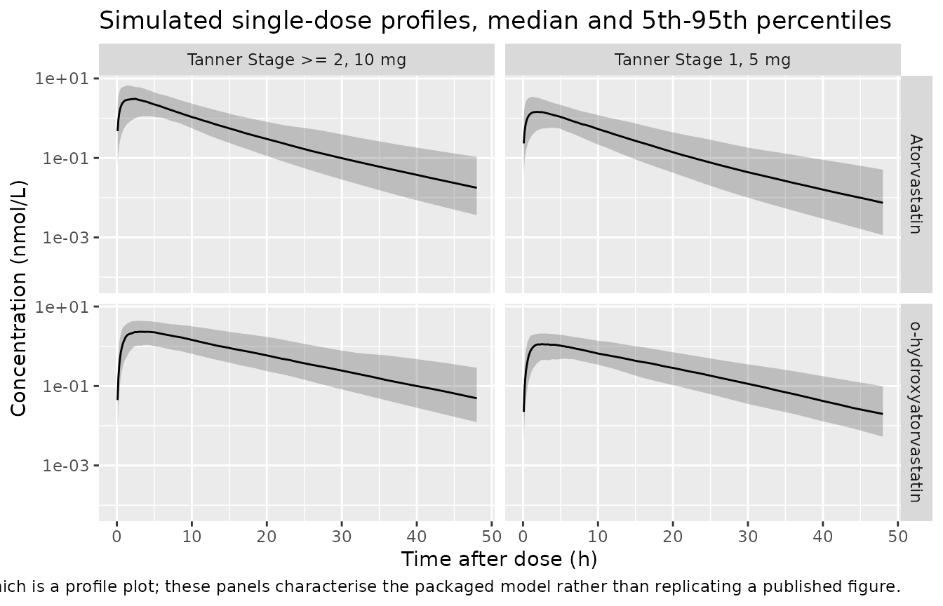
The two arms differ in exposure by more than the 2-fold dose ratio alone, because the Tanner Stage 1 arm is both lighter (lower CL/F) and has lower relative bioavailability.
PKNCA validation
One PKNCA block per analyte. The concentration filter is
!is.na(.) only: adding time > 0 or
conc > 0 would drop the time-zero anchor row.
run_nca <- function(sim, conc_col, events) {
  conc_df <- sim |>
    dplyr::filter(!is.na(.data[[conc_col]])) |>
    dplyr::transmute(id = sid, time, arm, conc = .data[[conc_col]]) |>
    # Keep conc >= 1e-6 * max(conc) per subject after the peak: below that it is solver noise.
    dplyr::group_by(id, arm) |>
    dplyr::filter(time <= time[which.max(conc)] | conc >= 1e-6 * max(conc)) |>
    dplyr::ungroup()

  # Guarantee a time = 0 row per (id, arm); pre-dose concentration is 0
  # for an extravascular single dose.
  conc_df <- dplyr::bind_rows(
    conc_df,
    conc_df |> dplyr::distinct(id, arm) |> dplyr::mutate(time = 0, conc = 0)
  ) |>
    dplyr::distinct(id, arm, time, .keep_all = TRUE) |>
    dplyr::arrange(id, arm, time)

  dose_df <- events |>
    dplyr::filter(evid == 1L) |>
    dplyr::transmute(id = sid, time, amt, arm)

  intervals <- data.frame(
    start = 0, end = Inf,
    cmax = TRUE, tmax = TRUE, aucinf.obs = TRUE, half.life = TRUE
  )

  PKNCA::pk.nca(PKNCA::PKNCAdata(
    PKNCA::PKNCAconc(conc_df, conc ~ time | arm + id),
    PKNCA::PKNCAdose(dose_df, amt ~ time | arm + id),
    intervals = intervals
  ))
}

nca_atv  <- run_nca(sim_vpc, "Cc",      events_vpc)
nca_oatv <- run_nca(sim_vpc, "Cc_oatv", events_vpc)
Per-subject AUC identity (exact closed form)
For a linear model with all elimination from the central compartment,
the single-dose AUC to infinity is exactly Dose * F1 / CL,
per subject. With fm fixed to 1 the whole atorvastatin
molar flux becomes o-ATV, so the metabolite obeys the same identity with
CLm/fm. Both sides use the same drawn parameters, so the
only difference is numerical – a tight bound is the correct assertion
here.
subj_params <- sim_vpc |>
  group_by(id = sid, arm) |>
  summarise(cl = first(cl), cl_oatv = first(cl_oatv), .groups = "drop") |>
  # The arm label carries the Tanner stratum, so F1 is recoverable without
  # depending on how rxSolve echoes the covariate column back.
  mutate(f1 = ifelse(grepl("Stage 1", arm, fixed = TRUE), f1_tan1, 1))
stopifnot(nrow(subj_params) == 2L * N_PER_ARM,
          dplyr::n_distinct(subj_params$f1) == 2L)

dose_by_id <- events_vpc |>
  filter(evid == 1L) |>
  transmute(id = sid, amt)

auc_check <- bind_rows(
  as.data.frame(nca_atv) |>
    filter(PPTESTCD == "aucinf.obs") |> mutate(analyte = "Atorvastatin"),
  as.data.frame(nca_oatv) |>
    filter(PPTESTCD == "aucinf.obs") |> mutate(analyte = "o-hydroxyatorvastatin")
) |>
  select(id, arm, analyte, auc_nca = PPORRES) |>
  left_join(subj_params, by = c("id", "arm")) |>
  left_join(dose_by_id, by = "id") |>
  mutate(
    clearance = ifelse(analyte == "Atorvastatin", cl, cl_oatv),
    auc_exact = amt * f1 / clearance,
    pct_diff  = 100 * (auc_nca - auc_exact) / auc_exact
  )

stopifnot(nrow(auc_check) == 4L * N_PER_ARM)

auc_check |>
  group_by(analyte, arm) |>
  summarise(
    n              = dplyr::n(),
    median_pct     = median(pct_diff),
    max_abs_pct    = max(abs(pct_diff)),
    .groups        = "drop"
  ) |>
  dplyr::rename(
    "Analyte"                       = analyte,
    "Arm"                           = arm,
    "N"                             = n,
    "Median difference (%)"         = median_pct,
    "Max absolute difference (%)"   = max_abs_pct
  ) |>
  knitr::kable(digits = 3,
caption = "PKNCA AUC(0-inf) vs. the exact Dose*F1/CL identity.")| Analyte | Arm | N | Median difference (%) | Max absolute difference (%) |
|---|---|---|---|---|
| Atorvastatin | Tanner Stage 1, 5 mg | 150 | -0.015 | 0.199 |
| Atorvastatin | Tanner Stage >= 2, 10 mg | 150 | -0.015 | 0.131 |
| o-hydroxyatorvastatin | Tanner Stage 1, 5 mg | 150 | 0.000 | 0.400 |
| o-hydroxyatorvastatin | Tanner Stage >= 2, 10 mg | 150 | 0.001 | 0.156 |
Terminal slope is the parent hybrid rate constant for both analytes
The metabolite’s own slowest hybrid rate constant (0.110 1/h at the
reference covariates) is faster than the parent’s L2
(0.0845 1/h), so o-ATV disposition should be
formation-rate-limited and both analytes should decay
with the parent’s terminal slope. Two instruments, used for what each is
good at.
Deterministic log-linear regression (the direct test)
Regressing log(concentration) on time over an
unambiguously terminal window measures the model’s terminal slope
directly, with no lambda_z point-selection heuristic in the way.
Typical-value profiles, so no seed and no cohort.
terminal_slope <- function(df, conc_col, lo = 48, hi = 72) {
  # Keep points >= 1e-6 * max: below that the ODE solution is integrator noise.
  d <- df[df$time >= lo & df$time <= hi & df[[conc_col]] >= 1e-6 * max(df[[conc_col]]), ]
  fit <- stats::lm(log(d[[conc_col]]) ~ d$time)
  c(k = -unname(coef(fit)[2]), r2 = summary(fit)$r.squared)
}

slopes <- lapply(split(sim_typ, sim_typ$arm), function(d) {
  atv  <- terminal_slope(d, "Cc")
  oatv <- terminal_slope(d, "Cc_oatv")
  tibble::tibble(
    arm     = d$arm[1],
    l2      = d$l2[1],
    k_atv   = atv[["k"]],  r2_atv  = atv[["r2"]],
    k_oatv  = oatv[["k"]], r2_oatv = oatv[["r2"]]
  )
}) |>
  bind_rows() |>
  mutate(
    pct_atv  = 100 * (k_atv  - l2) / l2,
    pct_oatv = 100 * (k_oatv - l2) / l2
  )

slopes |>
  dplyr::select(arm, l2, k_atv, pct_atv, k_oatv, pct_oatv) |>
  dplyr::rename(
    "Arm"                        = arm,
    "L2 (1/h)"                   = l2,
    "ATV terminal k (1/h)"       = k_atv,
    "ATV vs L2 (%)"              = pct_atv,
    "o-ATV terminal k (1/h)"     = k_oatv,
    "o-ATV vs L2 (%)"            = pct_oatv
  ) |>
  knitr::kable(digits = 5,
               caption = paste(
                 "Terminal log-linear slope over 48-72 h vs. the parent",
                 "hybrid rate constant L2."
))| Arm | L2 (1/h) | ATV terminal k (1/h) | ATV vs L2 (%) | o-ATV terminal k (1/h) | o-ATV vs L2 (%) |
|---|---|---|---|---|---|
| Tanner Stage >= 2, 10 mg | 0.09193 | 0.09218 | 0.27347 | 0.09089 | -1.12439 |
| Tanner Stage 1, 5 mg | 0.10050 | 0.10078 | 0.27623 | 0.09948 | -1.01600 |
stopifnot(
  # Both analytes decay at L2, to within 2% over this window. The o-ATV curve
  # is still asymptoting slightly at 48 h, which is why its residual (~1%) is
  # larger than the parent's (~0.3%).
  all(abs(slopes$pct_atv)  < 1),
  all(abs(slopes$pct_oatv) < 2),
  # Log-linearity over the window: anything below this would mean the chosen
  # window is not actually terminal, and the slope comparison would be
  # measuring the wrong thing.
  all(slopes$r2_atv  > 0.9999),
  all(slopes$r2_oatv > 0.9999)
)
PKNCA half-life, parent only
PKNCA’s automatic lambda_z point selection is a reliable instrument
for the parent here, and the per-subject half-life
tracks log(2)/L2 closely. It is not
reliable for o-ATV in this model: because the metabolite curve has a
long, shallow transition into the parent-driven terminal phase, the
automatic window lands pre-terminal for a minority of subjects and the
error reaches 110%. That is a limitation of the point-selection
heuristic on this curve shape, not of the model – the deterministic
regression above is the check that actually settles the o-ATV claim, so
the gate below deliberately covers the parent only.
hl <- as.data.frame(nca_atv) |>
  filter(PPTESTCD == "half.life") |>
  select(id, arm, half_life = PPORRES) |>
  left_join(
    sim_vpc |> group_by(id = sid, arm) |> summarise(l2 = first(l2), .groups = "drop"),
    by = c("id", "arm")
  ) |>
  mutate(
    half_life_exact = log(2) / l2,
    pct_diff        = 100 * (half_life - half_life_exact) / half_life_exact
  )

stopifnot(nrow(hl) == 2L * N_PER_ARM)

hl |>
  group_by(arm) |>
  summarise(n = dplyr::n(),
            median_pct  = median(pct_diff),
            q90_abs_pct = quantile(abs(pct_diff), 0.90),
            max_abs_pct = max(abs(pct_diff)),
            .groups = "drop") |>
  dplyr::rename(
    "Arm"                            = arm,
    "N"                              = n,
    "Median difference (%)"          = median_pct,
    "90th pctile absolute diff (%)"  = q90_abs_pct,
    "Max absolute difference (%)"    = max_abs_pct
  ) |>
  knitr::kable(digits = 3,
               caption = paste(
                 "PKNCA atorvastatin terminal half-life vs. log(2)/L2,",
                 "per subject."
))| Arm | N | Median difference (%) | 90th pctile absolute diff (%) | Max absolute difference (%) |
|---|---|---|---|---|
| Tanner Stage 1, 5 mg | 150 | -1.392 | 1.748 | 2.600 |
| Tanner Stage >= 2, 10 mg | 150 | -1.357 | 1.653 | 3.189 |
Mass balance with fm fixed to 1
With fm = 1 there is no competing atorvastatin
elimination route, so every absorbed molecule of atorvastatin must
appear as a molecule of o-ATV. Integrating the o-ATV elimination flux
over a long window recovers the bioavailable dose.
ev_mb <- make_events(1L, median_wt = 50, tanner_1 = 0L, dose_mg = 10,
                     arm = "mass balance",
                     obs_times = seq(0, 720, by = 0.5)) |>
  mutate(WT = 50)  # pin the exemplar weight so the printed numbers are stable
mb <- rxode2::rxSolve(ui_typical, events = ev_mb,
                      useLinCmt = FALSE) |>
  as.data.frame()
#> ℹ omega/sigma items treated as zero: 'etalcl', 'etalvc', 'etalcl_oatv'

# Cumulative o-ATV eliminated = integral of k30 * central_oatv dt.
k30_mb   <- unique(round(mb$k30, 10))
stopifnot(length(k30_mb) == 1L)
elim_mb  <- k30_mb * sum(diff(mb$time) *
                           (head(mb$central_oatv, -1) + tail(mb$central_oatv, -1)) / 2)

remaining <- with(tail(mb, 1),
                  depot + central + peripheral1 + central_oatv + peripheral1_oatv)
dose_avail <- mg_to_nmol(10, MW_ATV) * 1  # F1 = 1 for Tanner Stage >= 2

c(bioavailable_nmol = dose_avail,
  o_atv_eliminated_nmol = elim_mb,
  still_in_body_nmol = remaining,
  recovery_pct = 100 * (elim_mb + remaining) / dose_avail)
#>     bioavailable_nmol o_atv_eliminated_nmol    still_in_body_nmol
#>          1.790062e+04          1.789905e+04          8.580712e-25
#>          recovery_pct
#>          9.999127e+01

stopifnot(abs(100 * (elim_mb + remaining) / dose_avail - 100) < 0.5)
NCA summary
Knebel 2013 reports no NCA table – no Cmax, Tmax, AUC or half-life values for either analyte – so there is nothing to place beside these numbers from the paper. They are reported as a characterisation of the packaged model; the published-value comparison is the closed-form and Abstract-anchor set above.
bind_rows(
  as.data.frame(nca_atv)  |> mutate(analyte = "Atorvastatin"),
  as.data.frame(nca_oatv) |> mutate(analyte = "o-hydroxyatorvastatin")
) |>
  filter(PPTESTCD %in% c("cmax", "tmax", "aucinf.obs", "half.life")) |>
  group_by(analyte, arm, PPTESTCD) |>
  summarise(median = median(PPORRES), .groups = "drop") |>
  tidyr::pivot_wider(names_from = PPTESTCD, values_from = median) |>
  dplyr::rename(
    "Analyte"                = analyte,
    "Arm"                    = arm,
    "AUC0-inf (nM*h)"        = aucinf.obs,
    "Cmax (nM)"              = cmax,
    "t1/2 (h)"               = half.life,
    "Tmax (h)"               = tmax
  ) |>
  knitr::kable(digits = 3,
               caption = paste(
                 "Median simulated single-dose NCA parameters by arm.",
                 "No published comparator exists (see text)."
))| Analyte | Arm | AUC0-inf (nM*h) | Cmax (nM) | t1/2 (h) | Tmax (h) |
|---|---|---|---|---|---|
| Atorvastatin | Tanner Stage 1, 5 mg | 16.376 | 1.742 | 7.113 | 2.00 |
| Atorvastatin | Tanner Stage >= 2, 10 mg | 34.041 | 3.338 | 7.785 | 2.15 |
| o-hydroxyatorvastatin | Tanner Stage 1, 5 mg | 16.457 | 1.213 | 7.483 | 2.90 |
| o-hydroxyatorvastatin | Tanner Stage >= 2, 10 mg | 37.222 | 2.446 | 8.097 | 3.05 |
Steady-state accumulation
The trial dosed once daily for 8 weeks and sampled at Weeks 2, 4, 6 and 8, so all observations were at steady state. With a terminal half-life near 8.2 h and a 24 h interval, accumulation is modest.
The gate here is the superposition identity for a linear model: the
AUC over one dosing interval at steady state equals the
single-dose AUC to infinity,
Dose * F1 / CL. (The accumulation ratio – steady-state
interval AUC over the first interval’s AUC – is reported alongside but
not asserted; it is simply a function of the interval relative to the
half-life and has no published comparator.)
# Coarse grid over the run-up (the plot only needs the envelope), then a fine
# grid over the last interval so its AUC is resolved well enough to be
# compared against the closed form.
ss_times <- sort(unique(c(seq(0, 13 * 24, by = 1),
                          seq(13 * 24, 14 * 24, by = 0.1))))

ev_ss <- make_events(
  1L, median_wt = 50, tanner_1 = 0L, dose_mg = 10, arm = "10 mg q24h",
  obs_times = ss_times, dose_times = seq(0, 13 * 24, by = 24)
) |>
  mutate(WT = 50)

sim_ss <- rxode2::rxSolve(ui_typical, events = ev_ss,
                          useLinCmt = FALSE) |>
  as.data.frame()
#> ℹ omega/sigma items treated as zero: 'etalcl', 'etalvc', 'etalcl_oatv'

sim_ss |>
  # Drop the predose row only: Cc is 0 there.
  filter(time != 0) |>
  transmute(time, Atorvastatin = Cc, `o-hydroxyatorvastatin` = Cc_oatv) |>
  tidyr::pivot_longer(-time, names_to = "analyte", values_to = "conc") |>
  ggplot(aes(time / 24, conc, colour = analyte)) +
  geom_line() +
  labs(x = "Time (days)", y = "Concentration (nmol/L)", colour = NULL,
       title = "Typical-value profile, 10 mg atorvastatin once daily, 50 kg")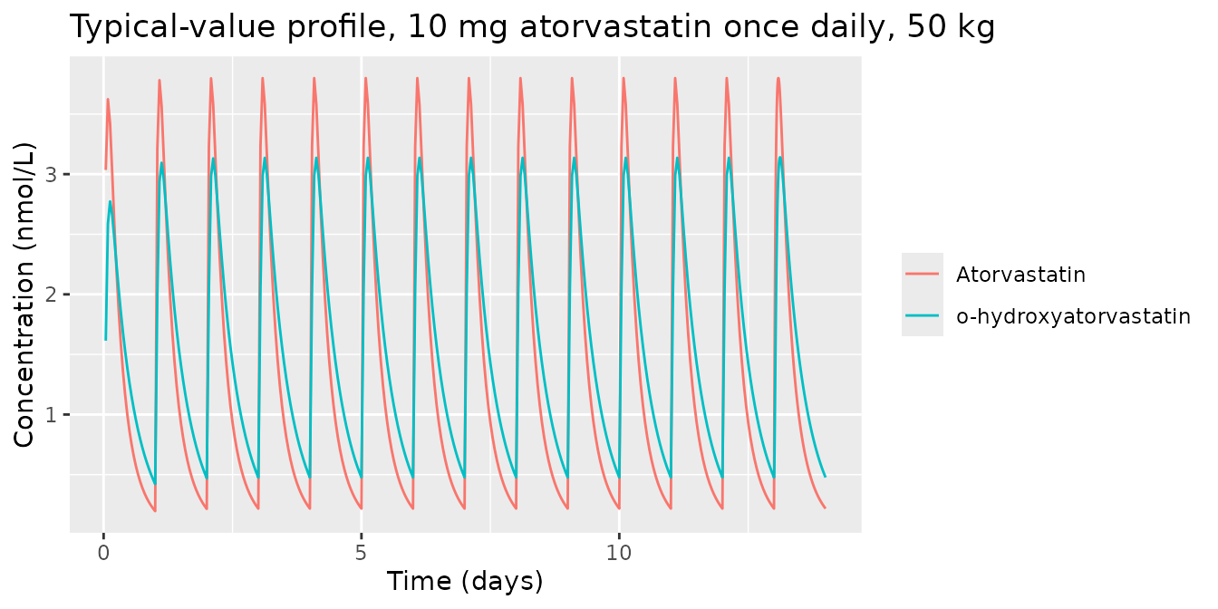
auc_interval <- function(df, lo, hi, col) {
  d <- df[df$time >= lo & df$time <= hi, ]
  sum(diff(d$time) * (head(d[[col]], -1) + tail(d[[col]], -1)) / 2)
}

# Superposition identity for a linear model: AUC over ONE dosing interval at
# steady state equals the SINGLE-dose AUC(0-inf), i.e. Dose * F1 / CL. This is
# an exact closed form on the same parameters, so it is the gate.
wt_ss   <- 50
cl_ss   <- exp(theta[["lcl"]])      * (wt_ss / 70)^theta[["e_wt_cl"]]
clm_ss  <- exp(theta[["lcl_oatv"]]) * (wt_ss / 70)^theta[["e_wt_cl_oatv"]]
dose_ss <- mg_to_nmol(10, MW_ATV)   # F1 = 1 for Tanner Stage >= 2

ss <- tibble::tibble(
  analyte   = c("Atorvastatin", "o-hydroxyatorvastatin"),
  auc_tau   = c(auc_interval(sim_ss, 13 * 24, 14 * 24, "Cc"),
                auc_interval(sim_ss, 13 * 24, 14 * 24, "Cc_oatv")),
  auc_exact = c(dose_ss / cl_ss, dose_ss / clm_ss),
  # Accumulation ratio: steady-state interval AUC over the FIRST interval's
  # AUC. Reported, not asserted -- it is a property of tau vs the half-life,
  # with no published comparator.
  acc_ratio = c(auc_interval(sim_ss, 13 * 24, 14 * 24, "Cc") /
                  auc_interval(sim_ss, 0, 24, "Cc"),
                auc_interval(sim_ss, 13 * 24, 14 * 24, "Cc_oatv") /
                  auc_interval(sim_ss, 0, 24, "Cc_oatv"))
) |>
  mutate(pct_diff = 100 * (auc_tau - auc_exact) / auc_exact)

ss |>
  dplyr::rename(
    "Analyte"                       = analyte,
    "AUC over interval 14 (nM*h)"   = auc_tau,
    "Dose * F1 / CL (nM*h)"         = auc_exact,
    "Difference (%)"                = pct_diff,
    "Accumulation ratio"            = acc_ratio
  ) |>
  knitr::kable(digits = 4,
               caption = paste(
                 "Steady-state interval AUC vs. the superposition closed form",
                 "Dose * F1 / CL, 10 mg once daily in a 50 kg patient."
))| Analyte | AUC over interval 14 (nM*h) | Dose * F1 / CL (nM*h) | Accumulation ratio | Difference (%) |
|---|---|---|---|---|
| Atorvastatin | 32.9555 | 32.960 | 1.0789 | -0.0136 |
| o-hydroxyatorvastatin | 37.4010 | 37.401 | 1.1446 | 0.0000 |
Assumptions and deviations
Q/F is taken as 227 L/h, not the 277 L/h printed in Table 2. Two independent places in the paper give 227: Supplemental Table S6, which is the per-run fixed-effect parameter log and lists Q/F = 227 for Run 340 (the run Table 2 is titled after), and the Discussion, which lists the final typical values as “699 L/hour (570, 881), 1020 L (209, 2210), 227 L/hour (80.2, 470), …”. Table S6’s neighbouring Run 356, which differs from Run 340 only in not fixing
fm, gives 223 L/h, close to 227 and not to 277. The bootstrap CI (80.2, 470) contains both candidates and so does not discriminate. A 227-to-277 digit transposition in typesetting is the parsimonious reading.Omega_1.1(CL/F IIV variance) is taken as 0.463^2 = 0.214, not the 0.124 printed in Table 2. The same Table 2 row states CV = 46.3%, and the paper’s convention throughout Tables 1 and 2 is CV% = 100 * sqrt(variance) (verified against all six Table 1 entries). sqrt(0.124) is 35.2%, not 46.3%; 0.463^2 = 0.214 reproduces the stated CV exactly. Independently, Supplemental Table S7 reports omega = 0.463 for ETA1 (CL/F) in Run 340. And 0.124 falls just below its own bootstrap 95% CI of (0.125, 0.293), whereas 0.214 sits inside it. Again a digit transposition (0.214 to 0.124).sigma_2.2bootstrap CI. Table 2 prints the o-ATV residual variance CI as (0.177, 0.207), which excludes its own point estimate of 0.166. The paper’s own “orthoATV CV” row gives the CI on the CV scale as (34.2, 45.5)%, i.e. (0.117, 0.207) as variances, so the lower bound is read as 0.117. This affects only the reported uncertainty, not the encoded point estimate.-
Ka reparameterisation: the printed equations contradict each other, and the model takes Equation S2 verbatim. Supplemental Equation S2 – the only equation printed for the final combined model – gives
Ka_i = exp(theta4 + L2_i), and that is what the model encodes. Two things in the paper pull against it:- Supplemental Equation S1, the earlier linear-scale parameterisation
of the same absorption model (which the paper says was
“carried forward as the ATV portion of the combined ATV/o-ATV
parent-metabolite model”), prints the purely additive
Ka_i = theta4 + L2_i. Its log-scale analogue isexp(theta4) + L2. - The main text states the purpose of the device as “The L2 was
calculated and incorporated into the calculation of Ka to avoid
‘flip-flop’ kinetics”, and only the additive form
achieves that purpose identically:
exp(theta4) + L2 > L2always, whereasexp(theta4 + L2)merely multiplies byexp(L2)and constrains nothing.
Consequence of the choice, for a typical Tanner-Stage-2-or-above 50 kg child (where
L2= 0.0919 1/h): the encoded Equation S2 reading givesKa= 0.219 1/h, while the additive reading givesKa= 0.292 1/h – about 28% higher atorvastatin Cmax and ~41% lower trough. The paper publishes no NCA table, no Tmax and no concentration-time figure with an absolute axis, so nothing in the available material discriminates the two. Equation S2 is used per the package’s convention that the printed equation has authority, because it is the only equation printed for the run the parameters come from (maintainer ruling). A user who prefers the additive reading need only change the singleka <- exp(lka + l2)line in the model file.A third reading exists: Tables 1 and 2 label the row “Ka = theta4”, so the paper itself sometimes treats 0.2 1/h as
Kaoutright, which would drop theL2term altogether. - Supplemental Equation S1, the earlier linear-scale parameterisation
of the same absorption model (which the paper says was
“carried forward as the ATV portion of the combined ATV/o-ATV
parent-metabolite model”), prints the purely additive
K30in Supplemental Equation S2 carries a spurious factor. Equation S2 prints the metabolite elimination rate constant asK30 = (CLm/fm) * fm_ATV / (Vcm/fm), reusing thefm_ATVfactor from theK20line immediately above it. Withfmfixed to 1 that factor is1 - fm = 0, soK30would be zero and o-ATV would never be eliminated – which is impossible, and is contradicted by the Figure 1 goodness-of-fit panels and byCLm/fmbeing estimated at 616 L/h with a tight CI. The factor is read as a copy-paste artifact and the model encodesK30 = (CLm/fm) / (Vcm/fm). The mass-balance check above is the gate on this reading.M3 censored likelihood is not reproduced. 16% of atorvastatin and 12% of o-ATV observations were below the 0.250 ng/mL limit of quantitation and were handled by Beal’s M3 method with
FOCEIL. nlmixr2 does not encode a censoring rule in the model object, so the model carries the proportional residual error the paper reports and any re-fit against censored data would need the censoring handled in the estimation call.Informative priors are estimation machinery, not model structure. The adult
PRIORhyperparameters (Equations 4 and 5) shaped the reported point estimates but are not part of the model definition and are not encoded. Note in passing that Equation 4’s printed prior modes for log(Q/F), log(Ka) and log(Vp/F) (4.29, -1.33, 7.07) do not back-transform to the corresponding adult estimates in Supplemental Table S4 (82 L/h, 0.0798 1/h, 1500 L); this internal inconsistency does not affect the final parameter values encoded here.fmfixed to 1 makes all metabolite parameters apparent. The paper is explicit that this was done for mathematical identifiability and that the resultingCLm/fm,Vcm/fm,Qm/fmandVpm/fm“are proportional to the ‘true’ values, adjusted by the fraction metabolized as proportionality constant”. They must not be read as absolute o-ATV disposition parameters. A consequence inside the model is thatK20(non-o-ATV atorvastatin elimination) is identically zero.p-hydroxyatorvastatin is not modelled, per the paper: it was below the limit of quantitation in over 80% of samples.
Cohort covariate distributions are assumed. Supplemental Table S1 reports only pooled weight and age; the per-Tanner-Stage weight distributions are “data not shown”. The arms above are anchored on the Abstract’s own 35 kg and 50 kg exemplars with 25% lognormal spread, truncated to the published 25-99.4 kg range. Sex and race are not reported and are not covariates in the model.
TANNER_1is a composite covariate. Tanner Stage 1 patients received 5 mg of a chewable tablet and Tanner Stage 2-or-above patients 10 mg of the marketed tablet, so dose level and formulation are confounded with the stage indicator; the paper says so explicitly and notes the 95% CI for the effect includes the null value of 1.Age was screened but not retained, and no coefficient was published, so it appears in
covariatesDataExcludedrather thancovariateData.No erratum or corrigendum was located for this article; the paper is subscription-access and no correction notice was found on the publisher landing page or in PubMed.