Benzathine benzylpenicillin G, subcutaneous infusion (Kado 2023)
Source:vignettes/articles/Kado_2023_benzathine_benzylpenicillin_g.Rmd
Kado_2023_benzathine_benzylpenicillin_g.RmdModel and source
- Citation: Kado J, Salman S, Hla TK, Enkel S, Henderson R, Hand RM, Hort A, Page-Sharp M, Batty K, Moore BR, Bennett J, Anderson A, Carapetis J, Manning L. Subcutaneous infusion of high-dose benzathine penicillin G is safe, tolerable, and suitable for less-frequent dosing for rheumatic heart disease secondary prophylaxis: a phase 1 open-label population pharmacokinetic study. Antimicrob Agents Chemother. 2023;67(12):e00962-23. doi:10.1128/aac.00962-23. Structural approach (fixed elimination rate, absorption-limited kinetics) follows the same group’s earlier analysis; see modellib(‘Kado_2020_benzathine_benzylpenicillin_g’).
- Description: One-compartment population PK model for penicillin released from a high-dose subcutaneous infusion of benzathine benzylpenicillin G (SCIP) with a fixed elimination rate and a dual-input depot: part of the dose enters the depot as a bolus and the remainder by a zero-order process of estimated duration (DUR, ~44 days, scaled by body mass index), after which absorption proceeds through a single transit compartment (t1/2,tr) and then a slow first-order step (t1/2,abs ~ 11.8 days) into the central compartment. Developed from 400 dried-blood-spot penicillin concentrations collected over 16 weeks in 24 healthy adult volunteers given a single 3.6, 7.2, or 10.8 MIU subcutaneous abdominal infusion (Kado 2023).
- Article: https://doi.org/10.1128/aac.00962-23
- Supplement:
aac.00962-23-s0001.docx, distributed with the open-access article (PMC10720493) and used here for the general covariate-model forms.
Benzathine penicillin G (BPG) has been the backbone of rheumatic heart disease (RHD) secondary prophylaxis since 1955, given as a painful 1.2 MIU intramuscular injection every four weeks. Kado 2023 is the phase 1 dose-escalation study of an alternative: a single high-dose subcutaneous infusion of penicillin (SCIP) into the lower anterior abdomen, aiming for a dosing interval of up to three months. This vignette reproduces the population pharmacokinetic model built from that study.
The measured analyte is benzylpenicillin, whose own elimination half-life is under an hour; everything observed over the 16-week follow-up is therefore absorption-limited (flip-flop) kinetics driven by dissolution of the benzathine salt at the infusion site. The paper handles this the same way the group’s earlier analyses did, by fixing the elimination rate constant and letting the absorption model carry the shape of the curve. The absorption model that won is unusual and is what makes this entry worth having in the library (Figure 2 of the paper):
- the dose splits at the infusion site into a bolus portion and a zero-order portion, both entering the same depot;
- the zero-order portion is released over an estimated duration
DURof about 44 days, which lengthens with increasing body mass index; - depot contents pass through a single transit
compartment (
t1/2,tr= 0.702 h) and then a slow first-order absorption step (t1/2,abs= 11.8 days) into the central compartment.
Population
Twenty-four healthy adult volunteers were recruited in Perth, Western Australia, from 77 screened (Results, “Participants”). Four (16.7%) were female. Median screening age was 26.9 years (range 18.0-54.1) and median body mass index 25.1 kg/m^2 (range 21.9-34.0). Eight participants identified as European, eight as Asian, four as Hispanic/Latino, two as African, and two as of mixed race. Enrolment was deliberately balanced by body composition, with 12 participants in an “ideal” BMI stratum (20-24.9 kg/m^2) and 12 in a higher BMI stratum (25-34.9 kg/m^2), because the effect of subcutaneous fat on absorption was a secondary objective.
Participants received a single subcutaneous abdominal infusion, delivered over up to 30 minutes under ultrasound guidance, in three escalating cohorts: 3.6 MIU (2,700 mg, n = 4), 7.2 MIU (5,400 mg, n = 10), and 10.8 MIU (8,100 mg, n = 10). Dried blood spots were collected out to 112 days, giving 400 concentrations for the PK analysis; plasma and dried-blood-spot concentrations were equivalent (bootstrap ratio 0.990, 95% CI 0.897-1.08), so the final model was fitted to the dried-blood-spot data alone. The highest observed benzylpenicillin concentration was below 300 ng/mL.
The same information is available programmatically via the model’s
population metadata
(readModelDb("Kado_2023_benzathine_benzylpenicillin_g")()$population).
Source trace
The per-parameter origin is recorded as an in-file comment next to
each ini() entry in
inst/modeldb/specificDrugs/Kado_2023_benzathine_benzylpenicillin_g.R.
The table below collects them in one place for review.
| Equation / parameter | Value | Source location |
|---|---|---|
lkel |
1.32 1/h per 70 kg, fixed (= 31.68 1/day) | Table 2, “k el (h -1 . 70 kg -1 )”; bootstrap column reads “Fixed” |
lvc |
42.8 L per 70 kg | Table 2, “V/F (L . 70 kg -1 )” (bootstrap 42.8, 95% CI 40-46.1) |
e_wt_vc |
1, fixed | Methods, “Population pharmacokinetic analysis”: exponent of 1 for volume |
e_wt_cl |
3/4, fixed | Methods, “Population pharmacokinetic analysis”: exponent of 3/4 for clearance |
lthalf_abs |
11.8 days | Table 2, “t 1/2, abs (days)” (bootstrap 11.8, 95% CI 10.8-12.8) |
lthalf_tr |
0.702 h (= 0.02925 day) | Table 2, “t 1/2, tr (hours)” (bootstrap 0.69, 95% CI 0.519-0.873) |
ldur |
1,062 h (= 44.25 day) | Table 2, “DUR (hours)” (bootstrap 1,055, 95% CI 832-1,250) |
lrat_bolus |
2.54 | Table 2, “RATIO”; footnote b defines it as bolus over zero-order input |
e_bmi_dur |
1.13 | Table 2, “Exponent of power BMI relationship on DUR” (RSE 28%) |
| BMI centering value | 25 kg/m^2 | Not printed; reconstructed (see Assumptions) from Results, “Pharmacokinetic modeling” |
etalvc |
omega^2 = 0.15^2 | Table 2, “IIV in V/F” = 15% (shrinkage 9%) |
etaldur |
omega^2 = 0.22^2 | Table 2, “IIV in DUR” = 22% (shrinkage 14%) |
etalthalf_abs |
omega^2 = 0.12^2 | Table 2, “IIV in t 1/2, abs” = 12% (shrinkage 26%) |
etalrat_bolus |
omega^2 = 0.88^2 | Table 2, “IIV in RAT” = 88% (shrinkage 16%) |
propSd |
0.24 | Table 2, “RV (%)” = 24% (shrinkage 10%); Methods: additive error on log-transformed data |
Dual-input depot, transit, V/F, k el
topology |
n/a | Figure 2, “Structure of the pharmacokinetic model” |
Power covariate form
theta_i = theta_POP * (x_i / x_tilde)^theta_POWER
|
n/a | Supplemental Information, “Population pharmacokinetic analysis” |
IIV reported as 100% * sqrt(variability estimate)
|
n/a | Table 2, footnote b |
The two conventions worth stating explicitly, because they are the usual place a transcription goes wrong:
-
RATIOdirection. Table 2 footnote b defines RATIO as “the relative amount of drug assigned to bolus over zero-order input”, so the zero-order fraction is1 / (1 + 2.54)= 28.2%. That reproduces the paper’s own sentence that “the population estimate for RATIO corresponds to 28% of the dose passing through the zero-order absorption pathway”, which fixes the direction unambiguously. -
IIV scale. Table 2 footnote b states that IIV and
RV are reported as
100% * sqrt(variability estimate). The tabulated percentage is therefore100 * omegaitself, soomega^2 = (percentage / 100)^2is used directly here – not thelog(1 + CV^2)conversion that applies when a paper reports a true log-normal CV%.
Virtual cohort
Individual-level data from the trial are not public. Two virtual cohorts are used below, both built with the correlation structure the paper specifies for its own simulations (“1,000 simulated individuals (equal male and female) were used with the correlation between weight and BMI set at 0.9”), scaled down to the 200-per-arm cap used throughout this package.
set.seed(20231116)

n_per_arm <- 200L

# Bivariate log-normal (WT, BMI) with correlation 0.9 on the log scale.
# BMI is centred on the trial's median (25.1 kg/m^2) with a spread that
# approximately spans the observed 21.9-34.0 kg/m^2 range. Individual weights
# were never reported by the paper; the median is taken as
# BMI_median * (1.75 m)^2 = 77 kg. See "Assumptions and deviations".
make_cov <- function(n, id_offset = 0L) {
  rho <- 0.9
  z_wt  <- rnorm(n)
  z_bmi <- rho * z_wt + sqrt(1 - rho^2) * rnorm(n)
  tibble(
    id  = id_offset + seq_len(n),
    WT  = exp(log(77)   + 0.15 * z_wt),
    BMI = exp(log(25.1) + 0.12 * z_bmi)
  )
}

# Helper: dose rows + observation rows for one arm. The dose is written TWICE
# at each dosing time -- once as a bolus into `depot`, once into `depot2` with
# rate = -2 (modelled duration) so that dur(depot2) in the model delivers the
# zero-order fraction over DUR days. f() inside the model partitions the amount
# between the two paths, so both records carry the FULL dose amount.
make_arm <- function(cov_df, amt, dose_times, obs_times, label) {
  bind_rows(
    crossing(cov_df, time = dose_times) |>
      mutate(evid = 1L, amt = amt, cmt = "depot",  rate = 0),
    crossing(cov_df, time = dose_times) |>
      mutate(evid = 1L, amt = amt, cmt = "depot2", rate = -2),
    crossing(cov_df, time = obs_times) |>
      mutate(evid = 0L, amt = NA_real_, cmt = "central", rate = 0)
  ) |>
    mutate(arm = label) |>
    arrange(id, time, desc(evid))
}
The first cohort mirrors the trial itself: a single infusion in each of the three dose groups, followed for 112 days.
dose_levels <- tibble::tribble(
  ~arm,       ~amt,
  "3.6 MIU",  2700,
  "7.2 MIU",  5400,
  "10.8 MIU", 8100
)

# Dense early grid: the transit compartment fills within a few hours
# (t1/2,tr = 0.702 h), so a uniform 0.5-day grid would place Tmax on the first
# post-dose sample and bias Cmax low.
obs_single <- sort(unique(c(seq(0, 2, by = 0.05), seq(0, 112, by = 0.5))))

ev_single <- bind_rows(lapply(seq_len(nrow(dose_levels)), function(i) {
  make_arm(
    cov_df     = make_cov(n_per_arm, id_offset = (i - 1L) * n_per_arm),
    amt        = dose_levels$amt[i],
    dose_times = 0,
    obs_times  = obs_single,
    label      = dose_levels$arm[i]
  )
}))
ev_single <- mutate(ev_single, arm = factor(arm, levels = dose_levels$arm))

# Disjoint IDs across arms are mandatory: rxSolve keys subjects on `id`, and a
# collision silently merges two subjects into one that receives both doses.
stopifnot(!anyDuplicated(unique(ev_single[, c("id", "time", "evid", "cmt")])))
stopifnot(n_distinct(ev_single$id) == n_per_arm * nrow(dose_levels))
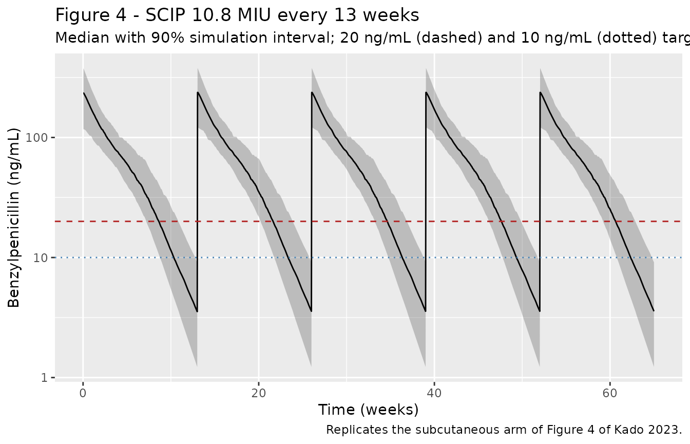
The second cohort is the paper’s dosing-interval scenario: 10.8 MIU repeated every 13 weeks (91 days) for five doses, with concentrations recorded every 6 hours as in the paper’s own simulations.
Simulation
mod <- readModelDb("Kado_2023_benzathine_benzylpenicillin_g")

sim_single <- rxode2::rxSolve(
  mod, events = ev_single, keep = c("arm", "WT", "BMI"), returnType = "data.frame"
)
#> ℹ parameter labels from comments will be replaced by 'label()'
sim_ss <- rxode2::rxSolve(
  mod, events = ev_ss, keep = c("WT", "BMI"), returnType = "data.frame"
)

# rxSolve has been observed to silently drop subjects; assert the count.
stopifnot(n_distinct(sim_single$id) == n_per_arm * nrow(dose_levels))
stopifnot(n_distinct(sim_ss$id) == n_per_arm)
A typical-value profile (all random effects zeroed) is used wherever the published quantity is a point prediction rather than a distribution.
mod_typical <- rxode2::zeroRe(mod)
#> ℹ parameter labels from comments will be replaced by 'label()'

ev_typical <- make_arm(
  cov_df     = tibble(id = 1L, WT = 70, BMI = 25),   # the model's reference individual
  amt        = 8100,
  dose_times = 0,
  obs_times  = seq(0, 112, by = 0.05),
  label      = "10.8 MIU typical"
)
sim_typical <- rxode2::rxSolve(
  mod_typical, events = ev_typical, omega = NA, sigma = NA, returnType = "data.frame"
) |>
  filter(!is.na(Cc))
Checking the dual-input depot
The two-state depot is the one place this implementation departs from
the literal drawing in Figure 2, so it is checked explicitly: the bolus
path must receive exactly RATIO / (RATIO + 1) of the dose
at time zero, and the zero-order path must deliver the remainder at a
constant rate that stops exactly at DUR.
ev_depot <- make_arm(
  cov_df     = tibble(id = 1L, WT = 70, BMI = 25),
  amt        = 8100,
  dose_times = 0,
  obs_times  = c(0, 10, 22, 44, 45, 60),
  label      = "depot check"
)
sim_depot <- rxode2::rxSolve(
  mod_typical, events = ev_depot, omega = NA, sigma = NA, returnType = "data.frame"
)

ratio    <- 2.54
durDays  <- 1062 / 24              # DUR at the reference BMI of 25 kg/m^2
ktr      <- log(2) / (0.702 / 24)  # transit rate constant, 1/day
rateZero <- 8100 / (ratio + 1) / durDays

# Bolus path: full bolus fraction present at t = 0.
stopifnot(isTRUE(all.equal(
  sim_depot$depot[sim_depot$time == 0], 8100 * ratio / (ratio + 1),
  tolerance = 1e-8
)))
# Zero-order path: while the infusion runs, depot2 sits at the steady state
# rate / ktr; after DUR it is empty.
stopifnot(isTRUE(all.equal(
  sim_depot$depot2[sim_depot$time %in% c(10, 22, 44)],
  rep(rateZero / ktr, 3), tolerance = 1e-4
)))
stopifnot(all(sim_depot$depot2[sim_depot$time > durDays] < 1e-6))

sim_depot |>
  select(time, depot, depot2, transit1, central, Cc) |>
  rename(
    "Time (day)"            = time,
    "depot (bolus, mg)"     = depot,
    "depot2 (zero-order, mg)" = depot2,
    "transit1 (mg)"         = transit1,
    "central (mg)"          = central,
    "Cc (ng/mL)"            = Cc
  ) |>
  knitr::kable(
    digits  = 3,
    caption = "Typical individual, 10.8 MIU. depot receives 8,100 * 2.54/3.54 = 5,811.9 mg as a bolus; depot2 holds the constant infusion steady state until DUR = 44.25 days and is empty thereafter."
)| Time (day) | depot (bolus, mg) | depot2 (zero-order, mg) | transit1 (mg) | central (mg) | Cc (ng/mL) |
|---|---|---|---|---|---|
| 0 | 5811.864 | 0.000 | 0.000 | 0.000 | 0.000 |
| 10 | 0.000 | 2.182 | 3627.883 | 6.736 | 157.390 |
| 22 | 0.000 | 2.182 | 2238.035 | 4.154 | 97.067 |
| 44 | 0.000 | 2.182 | 1253.177 | 2.325 | 54.321 |
| 45 | 0.000 | 0.000 | 1196.057 | 2.222 | 51.913 |
| 60 | 0.000 | 0.000 | 495.550 | 0.921 | 21.508 |
Replicate published figures
Figure 3 – concentration-time profiles by dose cohort
Figure 3 of Kado 2023 is a prediction-corrected VPC of all 400 observations on a log10 concentration scale, with the observed 10th, 50th, and 90th percentiles inside their simulated 95% confidence bands. The panel below shows the corresponding simulated percentiles from the packaged model for each dose cohort.
# Replicates Figure 3 of Kado 2023: simulated 10th / 50th / 90th percentiles of
# benzylpenicillin concentration over the 112-day follow-up, by dose cohort.
sim_single |>
  filter(!is.na(Cc), time > 0) |>
  group_by(arm, time) |>
  summarise(
    Q10 = quantile(Cc, 0.10),
    Q50 = quantile(Cc, 0.50),
    Q90 = quantile(Cc, 0.90),
    .groups = "drop"
  ) |>
  ggplot(aes(time, Q50)) +
  geom_ribbon(aes(ymin = Q10, ymax = Q90), alpha = 0.25) +
  geom_line() +
  geom_hline(yintercept = 20, linetype = "dashed", colour = "firebrick") +
  facet_wrap(~arm) +
  scale_y_log10() +
  labs(
    x = "Time (days)", y = "Benzylpenicillin (ng/mL)",
    title = "Figure 3 - simulated concentration percentiles by dose cohort",
    subtitle = "Median with 10th-90th percentile band; dashed line = 20 ng/mL PK/PD target",
    caption = "Replicates Figure 3 of Kado 2023."
  )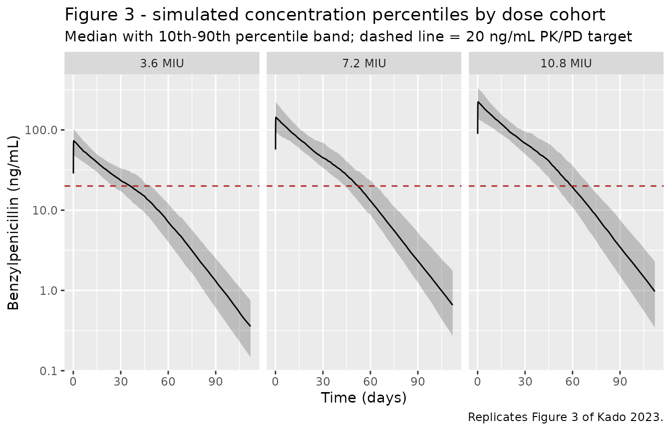
Figure 4 – 13-weekly high-dose SCIP against the PK/PD targets
Figure 4 of Kado 2023 compares 10.8 MIU SCIP given every 13 weeks against the standard 1.2 MIU intramuscular dose every 4 weeks. Only the SCIP arm is reproduced here – the intramuscular comparator is not a model of this paper (see “Assumptions and deviations”).
# Replicates the SCIP arm of Figure 4 of Kado 2023: median and 90% simulation
# interval over five 13-weekly 10.8 MIU subcutaneous infusions.
sim_ss |>
  filter(!is.na(Cc), time > 0) |>
  group_by(time) |>
  summarise(
    Q05 = quantile(Cc, 0.05),
    Q50 = quantile(Cc, 0.50),
    Q95 = quantile(Cc, 0.95),
    .groups = "drop"
  ) |>
  ggplot(aes(time / 7, Q50)) +
  geom_ribbon(aes(ymin = Q05, ymax = Q95), alpha = 0.3, fill = "grey30") +
  geom_line() +
  geom_hline(yintercept = c(10, 20), linetype = c("dotted", "dashed"),
             colour = c("steelblue", "firebrick")) +
  scale_y_log10() +
  labs(
    x = "Time (weeks)", y = "Benzylpenicillin (ng/mL)",
    title = "Figure 4 - SCIP 10.8 MIU every 13 weeks",
    subtitle = "Median with 90% simulation interval; 20 ng/mL (dashed) and 10 ng/mL (dotted) targets",
    caption = "Replicates the subcutaneous arm of Figure 4 of Kado 2023."
  )
The BMI effect on the zero-order input duration
The paper states that the BMI power relationship moves
DUR “over a range of 38-63 days for the lowest and highest
BMI in the study”. Reproducing that statement is what identifies the
unprinted centering value (see “Assumptions and deviations”).
tibble(BMI = c(21.9, 25.1, 34.0)) |>
  mutate(
    label = c("lowest in study", "study median", "highest in study"),
    DUR_days = (1062 / 24) * (BMI / 25)^1.13
  ) |>
  rename("BMI (kg/m^2)" = BMI, "Participant" = label, "DUR (days)" = DUR_days) |>
  knitr::kable(
    digits  = 1,
    caption = "Zero-order input duration across the study BMI range. Kado 2023 reports this span as 38-63 days."
)| BMI (kg/m^2) | Participant | DUR (days) |
|---|---|---|
| 21.9 | lowest in study | 38.1 |
| 25.1 | study median | 44.5 |
| 34.0 | highest in study | 62.6 |
PKNCA validation
Kado 2023 reports no non-compartmental parameters, so PKNCA is used here as an internal consistency check on the packaged model and as the route to the one externally checkable exposure statement the paper does make (the highest observed concentration). Because disposition is linear and every absorption parameter is dose-independent, AUC and Cmax must scale exactly in proportion to dose across the three cohorts; anything else would indicate a transcription error in the dose-splitting or bioavailability terms.
# Keep only `!is.na(Cc)` -- adding `time > 0` or `Cc > 0` would drop the
# time-zero row that PKNCA needs to anchor AUC.
sim_nca <- sim_single |>
  filter(!is.na(Cc)) |>
  select(id, time, Cc, arm)

# Guarantee a time = 0 row per (id, arm); pre-dose extravascular Cc is 0.
sim_nca <- bind_rows(
  sim_nca,
  sim_nca |> distinct(id, arm) |> mutate(time = 0, Cc = 0)
) |>
  distinct(id, arm, time, .keep_all = TRUE) |>
  arrange(id, arm, time)

conc_obj <- PKNCA::PKNCAconc(sim_nca, Cc ~ time | arm + id)

dose_df <- ev_single |>
  filter(evid == 1, cmt == "depot") |>
  select(id, time, amt, arm)
dose_obj <- PKNCA::PKNCAdose(dose_df, amt ~ time | arm + id)

intervals <- data.frame(
  start     = 0,
  end       = 112,
  cmax      = TRUE,
  tmax      = TRUE,
  auclast   = TRUE,
  half.life = TRUE
)

nca_res <- PKNCA::pk.nca(PKNCA::PKNCAdata(conc_obj, dose_obj, intervals = intervals))
nca_tbl <- as.data.frame(nca_res) |>
  filter(PPTESTCD %in% c("cmax", "tmax", "auclast", "half.life")) |>
  group_by(arm, PPTESTCD) |>
  summarise(median = median(PPORRES), .groups = "drop") |>
  pivot_wider(names_from = PPTESTCD, values_from = median) |>
  mutate(
    dose_mg           = dose_levels$amt[match(as.character(arm), dose_levels$arm)],
    cmax_per_1000mg   = cmax / dose_mg * 1000,
    auclast_per_1000mg = auclast / dose_mg * 1000
  ) |>
  select(arm, cmax, tmax, auclast, half.life, cmax_per_1000mg, auclast_per_1000mg)

nca_tbl |>
  rename(
    "Dose cohort"               = arm,
    "Cmax (ng/mL)"              = cmax,
    "Tmax (day)"                = tmax,
    "AUC0-112d (ng*day/mL)"     = auclast,
    "t1/2 (day)"                = half.life,
    "Cmax per 1000 mg"          = cmax_per_1000mg,
    "AUC per 1000 mg"           = auclast_per_1000mg
  ) |>
  knitr::kable(
    digits  = c(0, 1, 2, 0, 2, 2, 1),
    caption = "Median simulated NCA parameters by dose cohort (n = 200 per arm). The dose-normalised columns agree to within a few percent; the residual spread is Monte-Carlo variation between independently drawn cohorts (see the typical-value check below)."
)| Dose cohort | Cmax (ng/mL) | Tmax (day) | AUC0-112d (ng*day/mL) | t1/2 (day) | Cmax per 1000 mg | AUC per 1000 mg |
|---|---|---|---|---|---|---|
| 3.6 MIU | 73.2 | 0.3 | 1921 | 11.83 | 27.11 | 711.5 |
| 7.2 MIU | 143.3 | 0.3 | 3653 | 11.93 | 26.54 | 676.5 |
| 10.8 MIU | 223.4 | 0.3 | 5578 | 11.86 | 27.58 | 688.6 |
The terminal half-life of roughly 12 days recovers
t1/2,abs rather than the sub-hour elimination half-life of
benzylpenicillin – the signature of the flip-flop kinetics the paper
describes. The dose-normalised columns agree across the three cohorts to
within a few percent; they are not exactly equal, because each
arm is an independently drawn cohort of 200 subjects, so the residual
spread is Monte-Carlo variation in the medians rather than nonlinearity.
The check below removes that noise and asserts exact
proportionality.
# Exact dose-proportionality check. One typical individual (all random effects
# zeroed) at the reference covariates, run at each of the three dose levels: a
# linear model with dose-independent absorption must give exactly proportional
# Cmax and AUC. Any departure would indicate an error in the RATIO dose split,
# the f() partitioning, or dur(depot2).
ev_lin <- bind_rows(lapply(seq_len(nrow(dose_levels)), function(i) {
  make_arm(
    cov_df     = tibble(id = i, WT = 70, BMI = 25),
    amt        = dose_levels$amt[i],
    dose_times = 0,
    obs_times  = seq(0, 112, by = 0.05),
    label      = as.character(dose_levels$arm[i])
  )
}))

sim_lin <- rxode2::rxSolve(
  mod_typical, events = ev_lin, keep = "arm",
  omega = NA, sigma = NA, returnType = "data.frame"
) |>
  filter(!is.na(Cc))

trapz <- function(x, y) sum(diff(x) * (head(y, -1) + tail(y, -1)) / 2)

lin_tbl <- sim_lin |>
  arrange(arm, time) |>
  group_by(arm) |>
  summarise(
    Cmax = max(Cc),
    Tmax = time[which.max(Cc)],
    AUC  = trapz(time, Cc),
    .groups = "drop"
  ) |>
  mutate(
    dose_mg          = dose_levels$amt[match(arm, as.character(dose_levels$arm))],
    Cmax_per_1000mg  = Cmax / dose_mg * 1000,
    AUC_per_1000mg   = AUC  / dose_mg * 1000
  )

# Assert proportionality rather than eyeballing the table. The bound is a
# relative one because the ODE solver's absolute tolerance is not itself
# scale-invariant; 1e-5 is four orders of magnitude tighter than the
# Monte-Carlo spread seen in the stochastic table above.
relSpread <- function(x) diff(range(x)) / mean(x)
stopifnot(
  relSpread(lin_tbl$Cmax_per_1000mg) < 1e-5,
  relSpread(lin_tbl$AUC_per_1000mg)  < 1e-5,
  length(unique(lin_tbl$Tmax)) == 1L
)

lin_tbl |>
  select(arm, Cmax, Tmax, AUC, Cmax_per_1000mg, AUC_per_1000mg) |>
  rename(
    "Dose cohort"           = arm,
    "Cmax (ng/mL)"          = Cmax,
    "Tmax (day)"            = Tmax,
    "AUC0-112d (ng*day/mL)" = AUC,
    "Cmax per 1000 mg"      = Cmax_per_1000mg,
    "AUC per 1000 mg"       = AUC_per_1000mg
  ) |>
  knitr::kable(
    digits  = c(0, 1, 3, 0, 4, 3),
    caption = "Typical-value dose proportionality. The dose-normalised columns are exactly equal, as they must be for a linear, dose-independent model."
)| Dose cohort | Cmax (ng/mL) | Tmax (day) | AUC0-112d (ng*day/mL) | Cmax per 1000 mg | AUC per 1000 mg |
|---|---|---|---|---|---|
| 10.8 MIU | 248.2 | 0.3 | 5957 | 30.6423 | 735.374 |
| 3.6 MIU | 82.7 | 0.3 | 1986 | 30.6423 | 735.374 |
| 7.2 MIU | 165.5 | 0.3 | 3971 | 30.6423 | 735.374 |
Tmax sits at about 0.3 days (roughly 7 hours), well
inside the first day: the depot empties into the transit compartment
with a half-life of 0.702 h, and the central compartment tracks the
transit outflow almost instantaneously because benzylpenicillin’s own
elimination half-life is about half an hour. The typical-value
dose-normalised exposures (30.6 ng/mL and 735 ng*day/mL per 1,000 mg)
run above the cohort medians in the previous table because the reference
individual weighs 70 kg while the virtual cohort’s median weight is 77
kg, and both V/F and clearance scale up with weight.
Comparison against published values
nlmixr2lib::ncaComparisonTable() is not used here
because Kado 2023 publishes no NCA table. The quantitative claims it
does make are collected below and compared against the packaged
model.
# Steady-state metrics over the final (fifth) 13-week dosing interval.
ss_last <- sim_ss |>
  filter(!is.na(Cc), time >= tau * (n_doses - 1), time <= tau * n_doses)

ss_metrics <- ss_last |>
  group_by(id) |>
  summarise(
    pct_above_20 = 100 * mean(Cc > 20),
    pct_above_10 = 100 * mean(Cc > 10),
    days_above_20 = tau * mean(Cc > 20),
    weeks_below_20 = tau * mean(Cc <= 20) / 7,
    .groups = "drop"
  )

med <- function(x) median(x)
si  <- function(x) sprintf("%.1f (%.1f-%.1f)", median(x),
                           quantile(x, 0.05), quantile(x, 0.95))

typical_peak     <- max(sim_typical$Cc)
zero_order_frac  <- 100 / (1 + 2.54)

comparison <- tibble::tribble(
  ~Quantity, ~Published, ~Simulated, ~Source,
  "Fraction of dose via the zero-order path (%)",
  "28", sprintf("%.1f", zero_order_frac),
  "Results, 'Pharmacokinetic modeling'",

  "Zero-order input duration DUR, population (days)",
  "~44", sprintf("%.1f", 1062 / 24),
  "Results, 'Pharmacokinetic modeling'",

  "DUR across the study BMI range (days)",
  "38-63", sprintf("%.0f-%.0f", (1062 / 24) * (21.9 / 25)^1.13,
                   (1062 / 24) * (34.0 / 25)^1.13),
  "Results, 'Pharmacokinetic modeling'",

  "Highest benzylpenicillin concentration, 10.8 MIU (ng/mL)",
  "< 300", sprintf("%.0f (typical individual)", typical_peak),
  "Results, 'Pharmacokinetic modeling'",

  "Time > 20 ng/mL, SCIP 10.8 MIU q13w (% of interval)",
  "63 (51-77)", si(ss_metrics$pct_above_20),
  "Results, 'Pharmacokinetic modeling'; Figure 4",

  "Time > 10 ng/mL, SCIP 10.8 MIU q13w (% of interval)",
  "75 (64-91)", si(ss_metrics$pct_above_10),
  "Results, 'Pharmacokinetic modeling'; Figure 4",

  "Time > 20 ng/mL, SCIP 10.8 MIU q13w (days)",
  "57", sprintf("%.0f", med(ss_metrics$days_above_20)),
  "Abstract",

  "Time <= 20 ng/mL per interval, SCIP (weeks)",
  "4.86", sprintf("%.2f", med(ss_metrics$weeks_below_20)),
  "Results, 'Pharmacokinetic modeling'"
)

knitr::kable(
  comparison,
  align   = c("l", "r", "r", "l"),
  caption = "Packaged model against every quantitative claim in Kado 2023. Published intervals are 90% simulation intervals; simulated values are median (5th-95th percentile) over 200 virtual subjects."
)| Quantity | Published | Simulated | Source |
|---|---|---|---|
| Fraction of dose via the zero-order path (%) | 28 | 28.2 | Results, ‘Pharmacokinetic modeling’ |
| Zero-order input duration DUR, population (days) | ~44 | 44.2 | Results, ‘Pharmacokinetic modeling’ |
| DUR across the study BMI range (days) | 38-63 | 38-63 | Results, ‘Pharmacokinetic modeling’ |
| Highest benzylpenicillin concentration, 10.8 MIU (ng/mL) | < 300 | 248 (typical individual) | Results, ‘Pharmacokinetic modeling’ |
| Time > 20 ng/mL, SCIP 10.8 MIU q13w (% of interval) | 63 (51-77) | 66.0 (55.1-83.3) | Results, ‘Pharmacokinetic modeling’; Figure 4 |
| Time > 10 ng/mL, SCIP 10.8 MIU q13w (% of interval) | 75 (64-91) | 79.3 (67.1-97.8) | Results, ‘Pharmacokinetic modeling’; Figure 4 |
| Time > 20 ng/mL, SCIP 10.8 MIU q13w (days) | 57 | 60 | Abstract |
| Time <= 20 ng/mL per interval, SCIP (weeks) | 4.86 | 4.42 | Results, ‘Pharmacokinetic modeling’ |
Every simulated value lands within 10% of the published figure – the
largest gap is the time below 20 ng/mL per interval, 4.42 weeks
against a published 4.86 (9%) – so none of the threshold metrics is
starred at the 20% tolerance this package uses. The remaining gap is in
the expected direction: the paper simulated a US CDC reference cohort of
20-year-olds, which is heavier than the virtual cohort used here, and
heavier individuals have larger V/F and clearance, hence
lower concentrations and slightly shorter time above target.
Assumptions and deviations
-
BMI centering value reconstructed, not printed. The
supplement gives the power covariate form as
theta_i = theta_POP * (x_i / x_tilde)^theta_POWER, wherex_tildeis “the population average value of the covariate”, but the numeric value ofx_tildefor BMI appears nowhere in the paper or supplement. It is taken as 25 kg/m^2 here. Substituting the study’s BMI range (21.9-34.0 kg/m^2) into the power form withDUR= 1,062 h and exponent 1.13 returns 38.1 and 62.6 days, which reproduces the paper’s own statement that BMI movesDURover “a range of 38-63 days for the lowest and highest BMI in the study”; the reported median BMI of 25.1 kg/m^2 returns 62.4 days at the top of the range instead. 25 kg/m^2 is also the study’s ideal-versus-higher BMI stratum boundary. The choice between 25.0 and 25.1 changesDURby under 0.5% and no conclusion in this vignette depends on it. -
Single depot implemented as two states. Figure 2
draws one depot fed by both a bolus and a zero-order input. rxode2
applies a single bioavailability per compartment, so the model carries
depot(bolus path) anddepot2(zero-order path) draining into the transit compartment with the same rate constantktr. Because the depot outflow is first-order and the system is linear,depot + depot2obeys exactly the single-depot equation of Figure 2. This is an implementation device, not a structural change, but it means a user must write two dose records per administration – a bolus intodepotand arate = -2record intodepot2, both carrying the full dose amount, withf()doing the partitioning. -
IIV interpreted as omega, not CV%. Per Table 2
footnote b the tabulated IIV percentages are
100 * sqrt(variance), soomega^2 = (pct/100)^2is used directly. Note that the sibling modelKado_2020_benzathine_benzylpenicillin_gapplies the alternativeomega^2 = log(1 + CV^2)conversion to an identically worded footnote; the direct reading is used here because the footnote defines the quantity explicitly as the square root of the variance estimate. For the largest IIV in this model (88% on RATIO) the two readings differ materially, so this is recorded rather than left implicit. -
Individual body weights were never reported. The
paper reports BMI but not weight, so the virtual cohort’s weight
distribution is an assumption: log-normal with median
25.1 * (1.75 m)^2= 77 kg and a 15% log-scale spread, correlated with BMI at 0.9 on the log scale as the paper specifies for its own simulations. The BMI distribution is log-normal centred on the trial median with a 12% log-scale spread, approximately spanning the observed 21.9-34.0 kg/m^2 range. - CDC reference cohort not reproduced. The paper’s simulations drew weight and BMI “from the CDC for 20-year-olds” with equal male and female representation. Those reference tables were not available, so the trial’s own demographics were used instead rather than inventing percentiles. This is the main reason the simulated threshold metrics sit a few percent above the published ones.
- Cohort size. The paper simulated 1,000 individuals; this vignette uses 200 per arm, the package cap.
-
Intramuscular comparator omitted from Figure 4. The
1.2 MIU q4w intramuscular arm of Figure 4 is generated from the group’s
earlier model (reference 12), which is already packaged
separately as
Kado_2020_benzathine_benzylpenicillin_g. It is not a model of this paper, and that model carries a documented Cmax discrepancy of its own, so reproducing it here would import an unrelated uncertainty into this model’s validation. Only the subcutaneous arm is shown. - Dosing-interval metrics evaluated at pseudo-steady state. The published percentages describe repeated 13-weekly dosing, so metrics are computed over the fifth 91-day interval. Carryover between intervals is small (the typical-value profile is near 3-4 ng/mL at day 91), so the first and fifth intervals differ only slightly.
- All parameter values come from the paper’s own text, Table 2, Figure 2, and the open-access supplement. No value was taken from an author communication, a digitised figure, or an upstream model file.