Cefazolin (Santavy 2022) • nlmixr2lib

Model and source

#> ℹ parameter labels from comments will be replaced by 'label()'

Citation: Santavy P, Sima M, Zuscich O, Kubickova V, Michalickova D, Slanar O, Urbanek K. Population Pharmacokinetics of Prophylactic Cefazolin in Cardiac Surgery with Standard and Minimally Invasive Extracorporeal Circulation. Antibiotics (Basel). 2022;11(11):1582. doi:10.3390/antibiotics11111582
Description: Two-compartment population PK model for a prophylactic 2 g intravenous bolus of cefazolin in 65 adults undergoing cardiac surgery without cardiopulmonary bypass, with standard extracorporeal circulation (ECC) or with minimally invasive extracorporeal circulation (MiECC) (Santavy 2022). All covariate effects are exponential in the RAW, UNCENTERED covariate (Monolix log-linear form): CKD-EPI eGFR (per mL/s/1.73 m2) raises clearance, body surface area raises the central volume, and either type of bypass circuit lowers the peripheral volume relative to off-pump surgery. The model was fitted on a minute time scale; the published clearances (printed as L/h) are per minute and are converted here to L/h. Proportional residual error.
Article: https://doi.org/10.3390/antibiotics11111582 (open access)

Santavy et al. gave a single prophylactic 2 g intravenous bolus of cefazolin 30-60 min before cardiac surgery and sampled plasma richly through the operation. The final Monolix model has two compartments with first-order elimination. eGFR (CKD-EPI) acts on clearance, body surface area on the central volume, and the type of bypass circuit on the peripheral volume. Standard extracorporeal circulation (ECC) and minimally invasive extracorporeal circulation (MiECC) are each compared with off-pump surgery.

Population

Sixty-five adults were enrolled at University Hospital Olomouc, Czech Republic (Results 2.1, Table 1). Twenty had off-pump surgery (17 male), 25 were operated on MiECC (19 male) and 20 on standard ECC (19 male). Group medians were 68-73 years, 85-89 kg and a DuBois BSA of 1.98-2.01 m^2, with no significant between-group differences. Median CKD-EPI eGFR was 1.36-1.52 mL/s/1.73 m^2 (about 82-91 mL/min/1.73 m^2); Results 2.3 gives the range of the whole study as 0.67-2.8 mL/s. Surgery lasted a median 135 min off-pump, 198 min on ECC and 191 min on MiECC. Bypass ran a median 124 min on ECC and 71 min on MiECC. There were 461 plasma samples, taken at 15, 30, 45, 60, 120 and 180 min after the dose and at the end of surgery.

#> List of 13
#>  $ species       : chr "human"
#>  $ n_subjects    : int 65
#>  $ n_studies     : int 1
#>  $ n_observations: int 461
#>  $ age_range     : chr "44-86 years (group medians 68-73)"
#>  $ weight_range  : chr "51-117 kg (group medians 85-89)"
#>  $ sex_female_pct: num 15.4
#>  $ race_ethnicity: NULL
#>  $ disease_state : chr "Adults undergoing elective cardiac surgery: 20 off-pump, 25 on minimally invasive extracorporeal circulation (M"| __truncated__
#>  $ dose_range    : chr "Single 2 g intravenous bolus of cefazolin 30-60 min before the start of surgery"
#>  $ regions       : chr "Czech Republic (single centre: University Hospital Olomouc)"
#>  $ renal_function: chr "CKD-EPI eGFR group medians 1.36-1.52 mL/s/1.73 m^2 (about 82-91 mL/min/1.73 m^2); study range 0.67-2.8 mL/s (Re"| __truncated__
#>  $ notes         : chr "Prospective observational open-label PK study (Czech Health Research Council grant 17-31540A). Plasma sampled a"| __truncated__

Source trace

Every ini() value carries an in-file comment pointing to its source. The table collects them.

Equation / parameter	Value	Source location
`lcl`	`log(0.045 * 60)` = log(2.7 L/h)	Table 2, CL_pop = 0.045 (printed ‘L/h’, fitted per minute; see below)
`lvc`	`log(4.91)` L	Table 2, Vd1_pop
`lq`	`log(0.28 * 60)` = log(16.8 L/h)	Table 2, Q_pop = 0.28 (printed ‘L/h’, fitted per minute)
`lvp`	`log(22.07)` L	Table 2, Vd2_pop
`e_crcl_cl`	0.49 per mL/s/1.73 m^2	Table 2, beta_CL_eGFR
`e_bsa_vc`	0.51 per m^2	Table 2, beta_Vd1_BSA
`e_cpbstd_vp`	-0.77	Table 2, beta_Vd2_ECC
`e_cpbmini_vp`	-0.79	Table 2, beta_Vd2_MiECC
`etalcl`	0.35^2 = 0.1225	Table 2, omega_CL (SD)
`etalvc`	0.10^2 = 0.01	Table 2, omega_Vd1 (SD)
`etalq`	0.77^2 = 0.5929	Table 2, omega_Q (SD)
`etalvp`	0.58^2 = 0.3364	Table 2, omega_Vd2 (SD)
`propSd`	0.16	Table 2, ‘Proportional’
`cl`, `vc`, `q`, `vp` covariate equations	log-linear, uncentered	Table 2 footnote
Two-compartment ODE, IV bolus into `central`	n/a	Results 2.2; Methods 3.3
`crclSi <- CRCL / 60`	n/a	Table 1 reports eGFR in mL/s/1.73 m^2; the register column is mL/min/1.73 m^2

The time unit of the clearances

Table 2 labels CL_pop and Q_pop in L/h, but the fit was in minutes: samples were taken at 15-180 min, and the 407 min PTA horizon, the 215-318 min redosing times and the time axes of Figures 1-4 are all in minutes. The chunk below evaluates a typical patient both ways. Their eGFR is 1.42 mL/s, the cohort median, with a BSA of 1.99 m^2 and surgery on MiECC. No random numbers are involved.

egfr <- 1.42
bsa <- 1.99
cl_raw <- 0.045 * exp(0.49 * egfr)
vc_t <- 4.91 * exp(0.51 * bsa)
vp_t <- 22.07 * exp(-0.79)
q_raw <- 0.28
c407 <- function(cl, q, t) {
  # Closed-form two-compartment IV bolus, 2000 mg.
  k10 <- cl / vc_t
  k12 <- q / vc_t
  k21 <- q / vp_t
  s <- k10 + k12 + k21
  a <- (s + sqrt(s^2 - 4 * k10 * k21)) / 2
  b <- (s - sqrt(s^2 - 4 * k10 * k21)) / 2
  2000 / vc_t * ((a - k21) / (a - b) * exp(-a * t) + (k21 - b) / (a - b) * exp(-b * t))
}
unit_check <- tibble::tibble(
  reading = c("per minute (used here)", "per hour (as printed)"),
  `CL (L/h)` = c(cl_raw * 60, cl_raw),
  `Cc at 407 min (mg/L)` = c(c407(cl_raw, q_raw, 407), c407(cl_raw / 60, q_raw / 60, 407))
)
knitr::kable(unit_check, digits = 2)

reading	CL (L/h)	Cc at 407 min (mg/L)
per minute (used here)	5.41	17.25
per hour (as printed)	0.09	124.28

Read per minute, a typical patient clears 5.4 L/h, a usual cefazolin clearance in cardiac surgery, and is at about 17 mg/L 407 min after the dose. That is close to the 14-15 mg/L median of the middle panel of Figure 4, which spans eGFR 1-2.17 mL/s and all three circuits. Read per hour, clearance would be 0.09 L/h and the concentration would hardly fall over the operation. That contradicts every panel of Figure 4 and the redosing times the paper derives.

# Deterministic algebra, no RNG: a tight gate is appropriate. The x60
# conversion, a swapped beta or an additive reading of the covariate equations
# moves these by several-fold.
stopifnot(
  abs(unit_check$`CL (L/h)`[1] - 5.414) < 0.01,
  abs(unit_check$`Cc at 407 min (mg/L)`[1] - 17.25) < 0.05,
  unit_check$`Cc at 407 min (mg/L)`[2] > 100
)

Virtual cohort

The observed data are not public. The simulations below use virtual patients whose covariates follow Table 1. There are four arms of 200 patients each, matching the populations of Table 3 and Figure 4:

Study population. eGFR is log-normal with a median of 1.42 mL/s/1.73 m^2 (the mean of the three group medians) and log-SD 0.28, truncated to the study range 0.67-2.8 mL/s.
eGFR 0.67-1, 1-2.17 and 2.17-2.8 mL/s. These are the three panels of Figure 4. eGFR is uniform within each band. The last band is the “eGFR >= 2.17 mL/s” (augmented renal clearance) column of Table 3.

In every arm BSA is normal with mean 1.99 m^2 and SD 0.17, truncated to 1.58-2.46 m^2. The circuit is drawn with the enrolled proportions: 20 off-pump, 25 MiECC and 20 ECC out of 65.

# set.seed() seeds R's RNG (the covariate draw) only. rxode2's simulation RNG is
# partitioned per solver thread, so a CI runner with a different thread count
# draws different etas. Every assertion below is on a median or a proportion
# with a tolerance of at least 3 binomial standard errors, never on a tail value.
set.seed(20221109)
rxode2::rxSetSeed(20221109)

n_arm <- 200L
rtrunc_lnorm <- function(n, med, sdlog, lo, hi) {
  x <- numeric(0)
  while (length(x) < n) {
    y <- exp(rnorm(n, log(med), sdlog))
    x <- c(x, y[y >= lo & y <= hi])
  }
  x[seq_len(n)]
}
rtrunc_norm <- function(n, mean, sd, lo, hi) {
  x <- numeric(0)
  while (length(x) < n) {
    y <- rnorm(n, mean, sd)
    x <- c(x, y[y >= lo & y <= hi])
  }
  x[seq_len(n)]
}

make_cohort <- function(n, egfr, arm, id_offset) {
  circuit <- sample(c("off-pump", "MiECC", "ECC"), n, replace = TRUE, prob = c(20, 25, 20))
  tibble::tibble(
    id = id_offset + seq_len(n),
    arm = arm,
    eGFR = egfr,
    CRCL = egfr * 60,
    BSA = rtrunc_norm(n, 1.99, 0.17, 1.58, 2.46),
    SURG_CPB_STD = as.integer(circuit == "ECC"),
    SURG_CPB_MINI = as.integer(circuit == "MiECC")
  )
}

arms <- c("Study population", "eGFR 0.67-1", "eGFR 1-2.17", "eGFR 2.17-2.8")
subj <- dplyr::bind_rows(
  make_cohort(n_arm, rtrunc_lnorm(n_arm, 1.42, 0.28, 0.67, 2.8), arms[1], 0L),
  make_cohort(n_arm, runif(n_arm, 0.67, 1), arms[2], 1L * n_arm),
  make_cohort(n_arm, runif(n_arm, 1, 2.17), arms[3], 2L * n_arm),
  make_cohort(n_arm, runif(n_arm, 2.17, 2.8), arms[4], 3L * n_arm)
) |>
  dplyr::mutate(arm = factor(arm, levels = arms))
stopifnot(!anyDuplicated(subj$id))

# 2000 mg IV bolus at time 0 into the ODE state `central`. Observation rows also
# use cmt = "central"; Cc is returned as a column at those rows. Grid every
# 5 min to 405 min plus the 407 min PTA horizon, in hours (the model's unit).
t_obs_min <- sort(unique(c(seq(0, 405, by = 5), 407)))
dose_rows <- subj |>
  dplyr::mutate(time = 0, amt = 2000, evid = 1L, cmt = "central")
obs_rows <- subj |>
  tidyr::crossing(tmin = t_obs_min) |>
  dplyr::mutate(time = tmin / 60, amt = NA_real_, evid = 0L, cmt = "central") |>
  dplyr::select(-tmin)
events <- dplyr::bind_rows(dose_rows, obs_rows) |>
  dplyr::select(id, time, amt, evid, cmt, dplyr::everything()) |>
  dplyr::arrange(id, time, dplyr::desc(evid))
stopifnot(!anyDuplicated(events[, c("id", "time", "evid")]))

subj |>
  dplyr::group_by(arm) |>
  dplyr::summarise(
    n = dplyr::n(),
    `eGFR median (mL/s)` = median(eGFR),
    `BSA median (m^2)` = median(BSA),
    `ECC (%)` = 100 * mean(SURG_CPB_STD),
    `MiECC (%)` = 100 * mean(SURG_CPB_MINI)
  ) |>
  knitr::kable(digits = 2, caption = "Virtual cohort by arm.")

Virtual cohort by arm.
arm	n	eGFR median (mL/s)	BSA median (m^2)	ECC (%)	MiECC (%)
Study population	200	1.47	1.98	29.5	37.5
eGFR 0.67-1	200	0.81	1.99	36.0	34.0
eGFR 1-2.17	200	1.52	2.00	33.0	31.0
eGFR 2.17-2.8	200	2.47	1.99	32.5	39.5

Simulation

mod <- readModelDb("Santavy_2022_cefazolin")
sim <- rxode2::rxSolve(mod, events = events, keep = c("arm", "eGFR")) |>
  as.data.frame() |>
  dplyr::mutate(tmin = round(time * 60))
#> ℹ parameter labels from comments will be replaced by 'label()'
# `Cc` is the individual prediction (no residual error); `sim` adds the
# proportional residual error.
stopifnot(!anyNA(sim$Cc), all(sim$Cc >= -1e-6 * max(sim$Cc)))

Replicate published figures

Figure 3: visual predictive check

# Replicates Figure 3 of Santavy 2022: 10th, 50th and 90th percentiles of
# simulated concentrations (with residual error) for the study population.
# The paper's VPC replicates its own 65 patients; this one uses the virtual
# study-population arm.
vpc <- sim |>
  dplyr::filter(arm == "Study population", tmin >= 15) |>
  dplyr::group_by(tmin) |>
  dplyr::summarise(
    q10 = quantile(sim, 0.10),
    q50 = quantile(sim, 0.50),
    q90 = quantile(sim, 0.90),
    .groups = "drop"
  )
ggplot(vpc, aes(tmin)) +
  geom_ribbon(aes(ymin = q10, ymax = q90), fill = "steelblue", alpha = 0.25) +
  geom_line(aes(y = q50), colour = "steelblue4") +
  geom_line(aes(y = q10), colour = "steelblue", linetype = 2) +
  geom_line(aes(y = q90), colour = "steelblue", linetype = 2) +
  coord_cartesian(ylim = c(0, 180)) +
  labs(
    x = "Time (min)", y = "Cefazolin concentration (mg/L)",
    title = "Simulated 10th / 50th / 90th percentiles, 2 g IV bolus",
    caption = "Replicates Figure 3 of Santavy 2022."
  )

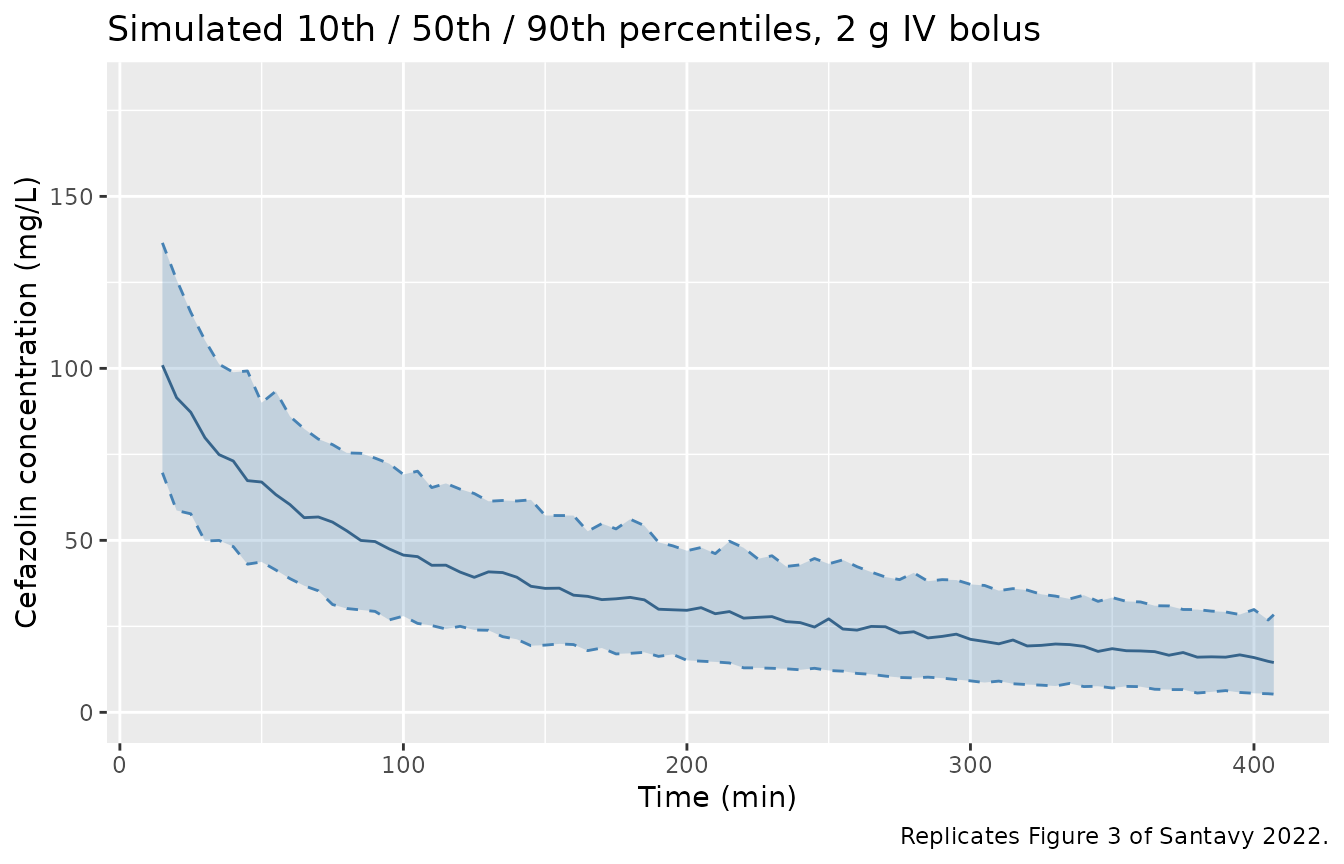
The observed median in Figure 3 falls from about 105 mg/L at 15 min to about 55 mg/L at 60 min and about 33 mg/L at 180 min. The 90th percentile is about 140 mg/L at 15 min, and the 10th percentile about 20 mg/L at 200 min. These values were read off the figure by the maintainers.

fig3 <- tibble::tribble(
  ~tmin, ~q50_fig,
  15, 105,
  60, 55,
  180, 33
)
fig3_cmp <- fig3 |>
  dplyr::left_join(vpc, by = "tmin") |>
  dplyr::mutate(pct_diff = 100 * (q50 / q50_fig - 1))
stopifnot(nrow(fig3_cmp) == 3, !anyNA(fig3_cmp$q50))
knitr::kable(fig3_cmp |> dplyr::select(tmin, q50_fig, q50, pct_diff), digits = 1)

tmin	q50_fig	q50	pct_diff
15	105	100.9	-3.9
60	55	60.4	9.8
180	33	33.4	1.3

# A median over 200 subjects is robust to which subjects land in the tails.
# A per-hour clearance (no decline), an additive covariate reading, or a
# Vd1/Vd2 swap moves these medians by far more than 25%.
stopifnot(all(abs(fig3_cmp$pct_diff) < 25))

Figure 4: profiles by renal function

# Replicates Figure 4 of Santavy 2022: median and 5-27.5-50-72.5-90th
# percentiles of simulated concentrations by eGFR band, with the 4 mg/L MIC.
fig4 <- sim |>
  dplyr::filter(arm != "Study population", tmin >= 15) |>
  dplyr::group_by(arm, tmin) |>
  dplyr::summarise(
    p05 = quantile(Cc, 0.05), p275 = quantile(Cc, 0.275),
    p50 = quantile(Cc, 0.50), p725 = quantile(Cc, 0.725),
    p90 = quantile(Cc, 0.90),
    .groups = "drop"
  )
ggplot(fig4, aes(tmin)) +
  geom_ribbon(aes(ymin = p05, ymax = p90), fill = "steelblue", alpha = 0.25) +
  geom_ribbon(aes(ymin = p275, ymax = p725), fill = "steelblue", alpha = 0.45) +
  geom_line(aes(y = p50)) +
  geom_hline(yintercept = 4, colour = "red") +
  facet_wrap(~arm) +
  coord_cartesian(ylim = c(0, 145)) +
  labs(
    x = "Time (min)", y = "Cefazolin concentration (mg/L)",
    caption = "Replicates Figure 4 of Santavy 2022."
  )

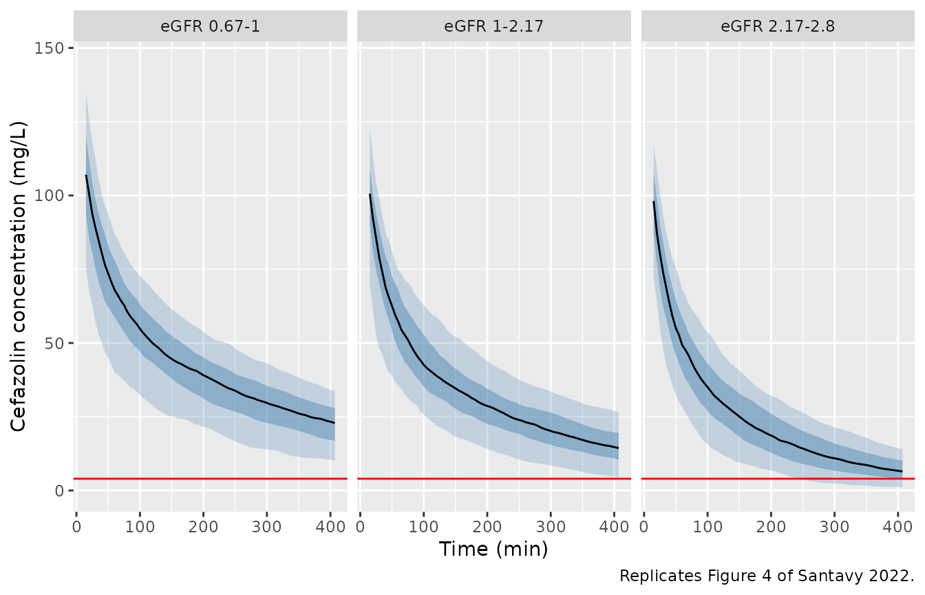
The Figure 4 medians at 407 min were read off the figure by the maintainers: about 23, 14.5 and 7.5 mg/L for the three bands.

fig4_ref <- tibble::tibble(
  arm = factor(arms[2:4], levels = arms),
  p50_fig = c(23, 14.5, 7.5)
)
fig4_cmp <- fig4 |>
  dplyr::filter(tmin == 407) |>
  dplyr::select(arm, p50) |>
  dplyr::inner_join(fig4_ref, by = "arm") |>
  dplyr::mutate(pct_diff = 100 * (p50 / p50_fig - 1))
stopifnot(nrow(fig4_cmp) == 3)
knitr::kable(fig4_cmp, digits = 1)

arm	p50	p50_fig	pct_diff
eGFR 0.67-1	22.9	23.0	-0.5
eGFR 1-2.17	14.4	14.5	-0.8
eGFR 2.17-2.8	6.5	7.5	-13.9

# The three bands differ about three-fold at 407 min, so a wrong sign or unit
# on the eGFR effect fails here immediately; 30% leaves room for digitising
# error and for a 200-subject median.
stopifnot(all(abs(fig4_cmp$pct_diff) < 30))

Probability of target attainment (Table 3)

The paper’s target is fT > MIC = 100% over the first 407 min. After a single bolus the concentration only falls, so the target is met when the concentration at 407 min exceeds the MIC. The PTA below uses individual predictions without residual error. The “eGFR < 2.17” column is the study-population arm restricted to eGFR < 2.17 mL/s.

mics <- c(0.25, 0.5, 1, 1.5, 2, 3, 4)
c407_df <- sim |> dplyr::filter(tmin == 407)
pta_of <- function(x) vapply(mics, function(m) 100 * mean(x > m), numeric(1))
study407 <- c407_df$Cc[c407_df$arm == "Study population"]
study_egfr <- c407_df$eGFR[c407_df$arm == "Study population"]
arc407 <- c407_df$Cc[c407_df$arm == "eGFR 2.17-2.8"]
stopifnot(length(study407) == n_arm, length(arc407) == n_arm)
pta <- tibble::tibble(
  MIC = mics,
  sim_all = pta_of(study407),
  pub_all = c(99.7, 99.5, 98.8, 98.1, 97.2, 95.1, 92.6),
  sim_lt = pta_of(study407[study_egfr < 2.17]),
  pub_lt = c(99.8, 99.5, 99.0, 98.3, 97.4, 95.5, 93.1),
  sim_arc = pta_of(arc407),
  pub_arc = c(97.9, 96.1, 92.4, 88.7, 84.7, 77.1, 69.7)
)
pta |>
  dplyr::rename(
    "MIC (mg/L)" = MIC,
    "Study, simulated" = sim_all, "Study, Table 3" = pub_all,
    "eGFR < 2.17, simulated" = sim_lt, "eGFR < 2.17, Table 3" = pub_lt,
    "eGFR >= 2.17, simulated" = sim_arc, "eGFR >= 2.17, Table 3" = pub_arc
  ) |>
  knitr::kable(digits = 1, caption = "PTA (%) for fT > MIC = 100% over 407 min.")

PTA (%) for fT > MIC = 100% over 407 min.
MIC (mg/L)	Study, simulated	Study, Table 3	eGFR < 2.17, simulated	eGFR < 2.17, Table 3	eGFR >= 2.17, simulated	eGFR >= 2.17, Table 3
0.2	100.0	99.7	100.0	99.8	99.5	97.9
0.5	100.0	99.5	100.0	99.5	97.5	96.1
1.0	99.0	98.8	98.9	99.0	95.0	92.4
1.5	98.5	98.1	98.4	98.3	91.5	88.7
2.0	98.5	97.2	98.4	97.4	88.0	84.7
3.0	97.5	95.1	97.4	95.5	80.5	77.1
4.0	94.5	92.6	94.7	93.1	71.0	69.7


# Binomial SE with 200 subjects: about 1.9 points at a PTA of 92% and 3.2 points
# at 70%. The bounds are more than 3 SE wide and still fail when CL and Q are
# read per hour, which gives 100% at every MIC.
stopifnot(
  max(abs(pta$sim_all - pta$pub_all)) < 8,
  max(abs(pta$sim_arc - pta$pub_arc)) < 15,
  pta$sim_arc[pta$MIC == 4] < 90
)

Redosing times for augmented renal clearance

Results 2.3 recommends a second dose in augmented renal clearance (eGFR >= 2.17 mL/s) at 215, 245, 288 and 318 min for MICs of 4, 3, 2 and 1.5 mg/L. Those are the times when the 10th percentile of concentrations reaches the MIC. The table gives the simulated crossing times with and without residual error. A blank cell means the 10th percentile is still above the MIC at 407 min.

arc_q10 <- sim |>
  dplyr::filter(arm == "eGFR 2.17-2.8", tmin >= 15) |>
  dplyr::group_by(tmin) |>
  dplyr::summarise(
    q10_ipred = quantile(Cc, 0.10),
    q10_ruv = quantile(sim, 0.10),
    .groups = "drop"
  )
cross_time <- function(mic, q10) {
  # Interpolate the first crossing of the MIC on the log scale.
  i <- which(q10 <= mic)[1]
  if (is.na(i)) {
    return(NA_real_)
  }
  t0 <- arc_q10$tmin[i - 1]
  t1 <- arc_q10$tmin[i]
  y0 <- log(q10[i - 1])
  y1 <- log(q10[i])
  t0 + (log(mic) - y0) / (y1 - y0) * (t1 - t0)
}
redose_mic <- c(4, 3, 2, 1.5)
redose <- tibble::tibble(
  `MIC (mg/L)` = redose_mic,
  `Results 2.3 (min)` = c(215, 245, 288, 318),
  `Simulated, no residual error (min)` = vapply(redose_mic, cross_time, numeric(1), q10 = arc_q10$q10_ipred),
  `Simulated, with residual error (min)` = vapply(redose_mic, cross_time, numeric(1), q10 = arc_q10$q10_ruv)
)
knitr::kable(redose, digits = 0)

MIC (mg/L)	Results 2.3 (min)	Simulated, no residual error (min)	Simulated, with residual error (min)
4	215	289	285
3	245	326	322
2	288	374	383
2	318	NA	NA

# Known deviation, not gated against the published times (see below). The gate
# checks only that the 10th percentile of the augmented-renal-clearance arm
# reaches 4 mg/L inside the 407 min window, which Table 3 (PTA 69.7% at 4
# mg/L) requires and a per-hour clearance would not produce.
stopifnot(
  !is.na(redose$`Simulated, no residual error (min)`[1]),
  redose$`Simulated, no residual error (min)`[1] < 407
)

The simulated times are later than the published ones by about 1 to 1.5 h. This is a known deviation, and the published times do not agree with the paper’s own Table 3. Table 3 gives a PTA of 88.7% at 1.5 mg/L over 407 min in the same population, so about 11% of patients are below 1.5 mg/L at 407 min. The 10th percentile therefore crosses 1.5 mg/L shortly before 407 min, not at 318 min. In the same way, a PTA of 69.7% at 4 mg/L puts the 10th-percentile crossing well before 407 min, but nothing in Table 3 supports one as early as 215 min. The model reproduces Table 3, as shown above. The paper does not say how its redosing times were derived, and they are not used to judge the model.

PKNCA validation

The paper reports no non-compartmental results. NCA on the simulated profiles gives the exposure per eGFR band over the 407 min horizon. The terminal half-life comes from the last part of that window and so describes the operative period, not the full washout.

sim_nca <- sim |>
  dplyr::filter(!is.na(Cc)) |>
  dplyr::select(id, time, Cc, arm)
conc_obj <- PKNCA::PKNCAconc(sim_nca, Cc ~ time | arm + id)
dose_df <- events |>
  dplyr::filter(evid == 1) |>
  dplyr::select(id, time, amt, arm)
dose_obj <- PKNCA::PKNCAdose(dose_df, amt ~ time | arm + id, route = "intravascular")
intervals <- data.frame(
  start = 0,
  end = 407 / 60,
  cmax = TRUE,
  auclast = TRUE,
  clast.obs = TRUE,
  half.life = TRUE
)
nca_res <- PKNCA::pk.nca(PKNCA::PKNCAdata(conc_obj, dose_obj, intervals = intervals))
nca_summary <- as.data.frame(nca_res$result) |>
  dplyr::filter(PPTESTCD %in% c("cmax", "auclast", "clast.obs", "half.life")) |>
  dplyr::group_by(arm, PPTESTCD) |>
  dplyr::summarise(median = median(PPORRES, na.rm = TRUE), .groups = "drop") |>
  tidyr::pivot_wider(names_from = PPTESTCD, values_from = median)
nca_summary |>
  dplyr::rename(
    "Arm" = arm,
    "Cmax (mg/L)" = cmax,
    "AUC0-407min (mg*h/L)" = auclast,
    "C at 407 min (mg/L)" = clast.obs,
    "t1/2 (h)" = half.life
  ) |>
  knitr::kable(digits = 2, caption = "Median simulated NCA by arm.")

Median simulated NCA by arm.
Arm	AUC0-407min (mg*h/L)	C at 407 min (mg/L)	Cmax (mg/L)	t1/2 (h)
Study population	257.85	15.49	149.23	3.62
eGFR 0.67-1	315.38	22.87	150.35	4.70
eGFR 1-2.17	243.72	14.38	147.47	3.92
eGFR 2.17-2.8	190.92	6.46	147.52	2.35

stopifnot(!anyNA(nca_summary$auclast))
# AUC must fall as eGFR rises; the 2.17-2.8 band has about 1.9-fold the
# clearance of the 0.67-1 band.
auc_lo <- nca_summary$auclast[nca_summary$arm == "eGFR 0.67-1"]
auc_hi <- nca_summary$auclast[nca_summary$arm == "eGFR 2.17-2.8"]
stopifnot(auc_lo / auc_hi > 1.2)

Assumptions and deviations

Clearance time unit. Table 2 prints CL_pop = 0.045 and Q_pop = 0.28 in L/h. The model was fitted with time in minutes, so the maintainers read both values per minute and multiplied them by 60 (2.7 and 16.8 L/h). The per-minute reading reproduces Table 3, Figure 4 and the redosing times above. The per-hour reading gives a clearance of 0.09 L/h and a PTA of 100% at every MIC.
Covariate equations. The Table 2 footnote gives the Monolix log-linear form, log(P) = log(P_pop) + beta * covariate, with uncentered covariates. The model uses this form. The Abstract and Discussion read the coefficients additively (“increased by 0.49 L/h with each 1 mL/s/1.73 m^2”, “a central Vd of 5.79 L in a patient with a BSA of 1.73 m^2”, “reduction in Vd by only 3.5%”). That reading is not used. Under the printed equation, the typical central volume at a BSA of 1.73 m^2 is 4.91 x exp(0.51 x 1.73) = 11.9 L, and either bypass circuit lowers the peripheral volume by about 54%, not 3.5%. The additive reading of the clearance gives 0.74 L/h (per hour) or 44 L/h (per minute) at the median eGFR. Neither is compatible with Figure 4.
eGFR units. Table 1, Results 2.3 and the Discussion give eGFR in mL/s/1.73 m^2; the Abstract’s “mL/min/1.73 m^2” is a misprint. The model’s CRCL column is in mL/min/1.73 m^2 and is divided by 60 inside the model.
Table 1 misprint. The ECC-group eGFR range is printed as “1.36 (1.68-1.85)”, which does not contain its own median. It is not used.
Bypass circuit covariates. SURG_CPB_STD (standard ECC) and SURG_CPB_MINI (MiECC) are subject-level indicators of the circuit used for the operation. The maintainers registered them as new canonical columns. They are distinct from the time-varying intra-operative windows CPB_ON / CPB_REWARM / CPB_POST. The paper applies the effect to every observation of a patient, including those before bypass started.
Virtual cohort. The paper gives eGFR only as group medians and ranges, so the study-population eGFR distribution (log-normal, median 1.42, log-SD 0.28, truncated to 0.67-2.8 mL/s) was chosen by the maintainers. Uniform distributions were used within the Figure 4 bands. BSA is normal around the Table 1 medians. Covariates were drawn independently.
Figure values. The Figure 3 medians and Figure 4 medians at 407 min were read off the published figures by the maintainers and are approximate.
Redosing times not reproduced. The 215-318 min redosing times of Results 2.3 come out 1 to 1.5 h later in the simulation. They are inconsistent with the paper’s Table 3, which the model does reproduce, so they are shown but not used to judge the model.
PTA without residual error. The simulated PTA uses individual predictions. The paper does not say whether its Simulx simulations included residual error.
No erratum or correction notice for this article was found in Crossref or Europe PMC as of 2026-10-15.