Piperacillin (Obrink-Hansen 2015)
Source:vignettes/articles/ObrinkHansen_2015_piperacillin.Rmd
ObrinkHansen_2015_piperacillin.RmdModel and source
- Citation: Obrink-Hansen K, Juul RV, Storgaard M, Thomsen MK, Hardlei TF, Brock B, Kreilgaard M, Gjedsted J. Population pharmacokinetics of piperacillin in the early phase of septic shock: does standard dosing result in therapeutic plasma concentrations? Antimicrob Agents Chemother. 2015;59(11):7018-7026. doi:10.1128/AAC.01347-15.
- Description: Two-compartment population PK model for piperacillin in critically ill adults with septic shock (Obrink-Hansen 2015); linear first-order elimination with an additive linear effect of plasma creatinine on clearance, IIV on CL and central volume, and a proportional residual error.
- Article: https://doi.org/10.1128/AAC.01347-15
Population
Obrink-Hansen et al. 2015 developed a population PK model of piperacillin in 15 critically ill adults with known or suspected septic shock requiring noradrenaline infusion, admitted to the Intensive Care Unit at Aarhus University Hospital (Skejby, Denmark) between September 2014 and January 2015 (ClinicalTrials.gov NCT02306928). Eligible patients were treated empirically with piperacillin-tazobactam (4 g / 0.5 g) given every 8 hours as a 3-minute intravenous infusion; patients on renal replacement therapy and those under 18 years were excluded. Sampling was performed during the third consecutive dose: eight free-piperacillin plasma concentrations per patient (predose; 10, 20, 30 minutes; 1, 2, 4, and 8 hours after the start of the third infusion) were quantified by UHPLC after 30 kDa ultrafiltration. Baseline characteristics (Obrink-Hansen 2015 Table 1): age median 66 years (IQR 59-79), 11 men and 4 women, body weight median 80 kg (IQR 70.2-95), plasma creatinine median 170 umol/L (IQR 119-282; observed range 53-446), plasma albumin median 30 g/L (IQR 27-32), APACHE score median 19 (IQR 14-23), SOFA score median 9 (IQR 7-10), and noradrenaline infusion rate median 0.1 ug/kg/min (IQR 0.04-0.24). Acute kidney injury was documented in 10 of 15 patients (67%).
The same metadata is available programmatically via
readModelDb("ObrinkHansen_2015_piperacillin")()$population.
Source trace
The per-parameter origin is recorded inline next to each
ini() entry in
inst/modeldb/specificDrugs/ObrinkHansen_2015_piperacillin.R.
The table below collects them in one place for review.
| Equation / parameter | Value | Source location |
|---|---|---|
lcl (CL, L/h) at CREAT = 170 umol/L |
log(3.6) |
Obrink-Hansen 2015 Table 2: CL 3.6 L/h (RSE 15.7%) |
lvc (V1, L) |
log(7.3) |
Obrink-Hansen 2015 Table 2: V1 7.3 L (RSE 11.8%) |
lq (Q, L/h) |
log(6.58) |
Obrink-Hansen 2015 Table 2: Q 6.58 L/h (RSE 16.4%) |
lvp (V2, L) |
log(3.9) |
Obrink-Hansen 2015 Table 2: V2 3.9 L (RSE 9.7%) |
e_creat_cl (beta_Pcrea on CL, (L/h)/(umol/L)) |
-0.011 |
Obrink-Hansen 2015 Table 2: beta_Pcrea -0.011 (RSE 11.9%) |
creat_ref (cohort median CREAT, umol/L) |
170 |
Obrink-Hansen 2015 Table 1 cohort median; Table 2 footnote |
etalcl (omega^2 on CL) |
0.41001 (71.2% CV) |
Obrink-Hansen 2015 Table 2: IIV CL 71.2% CV; omega^2 = log(1 + CV^2) |
etalvc (omega^2 on V1) |
0.28818 (57.8% CV) |
Obrink-Hansen 2015 Table 2: IIV V1 57.8% CV; omega^2 = log(1 + CV^2) |
propSd (proportional residual SD) |
0.147 |
Obrink-Hansen 2015 Table 2: proportional error 14.7% (RSE 14.4%) |
Covariate model (additive linear):
CL_i = (TVCL + beta_Pcrea * (CREAT - 170)) * exp(eta_CL)
|
n/a | Obrink-Hansen 2015 Table 2 footnote |
d/dt(central) and d/dt(peripheral1) (2-cmt
IV, linear elimination) |
n/a | Obrink-Hansen 2015 Results: “best described by a two-compartment model with linear elimination” |
| Proportional residual error | n/a | Obrink-Hansen 2015 Results: “Residual variability was best described by a proportional residual error model” |
Virtual cohort
Original observed concentrations are not publicly available. The simulations below use a virtual cohort whose plasma-creatinine distribution mirrors the Obrink-Hansen 2015 Table 1 cohort summary: 1000 subjects with serum creatinine drawn from a log-normal distribution targeting the published median (170 umol/L) and IQR (119-282 umol/L), truncated to the observed cohort range (53-446 umol/L).
set.seed(2015)

# Dose, infusion duration, and dose-interval per Obrink-Hansen 2015 Methods:
# "Piperacillin-tazobactam (4 g/0.5 g) was administered as a 3-min infusion
# intravenously (i.v.) every 8 h."
DOSE_MG       <- 4000     # mg piperacillin per dose
T_INF         <- 3 / 60   # hours: 3-min infusion
DOSE_INTERVAL <- 8        # hours between doses
N_DOSES       <- 3        # third dosing interval is the sampled / NCA interval
N_SUBJ        <- 1000L

# Plasma creatinine: log-normal that recovers median = 170 and IQR = 119-282.
# meanlog = log(170); sdlog from the IQR width: IQR(logN) = 1.349 * sdlog,
# so sdlog = log(282 / 119) / 1.349 = 0.640. Truncate to observed range
# (53-446 umol/L) to avoid extrapolation outside the cohort.
creat_med <- 170
sdlog     <- log(282 / 119) / 1.349

cohort <- tibble(
  id    = seq_len(N_SUBJ),
  CREAT = pmin(pmax(rlnorm(N_SUBJ, meanlog = log(creat_med), sdlog = sdlog),
                    53), 446)
)

# Build one subject's event table: three 4 g IV infusions at t = 0, 8, 16 h
# and a dense observation grid bracketing the third interval (16-24 h) for
# steady-state NCA of Cmax, Cmin, AUC0-8, and terminal half-life.
make_subject <- function(id, CREAT) {
  dose_times <- (seq_len(N_DOSES) - 1L) * DOSE_INTERVAL
  ev <- rxode2::et(
    amt   = DOSE_MG,
    rate  = DOSE_MG / T_INF,
    cmt   = "central",
    time  = dose_times
  )
  # Dense observation grid: every 6 min through 24 h, plus the exact
  # post-infusion sampling lattice the paper used during the third dose
  # (10, 20, 30 min; 1, 2, 4, 8 h after the start of the third infusion).
  obs_grid <- sort(unique(c(
    seq(0, 3 * DOSE_INTERVAL, by = 0.1),
    2 * DOSE_INTERVAL + c(0, 10/60, 20/60, 30/60, 1, 2, 4, 8)
  )))
  ev <- rxode2::et(ev, obs_grid)
  df <- as.data.frame(ev)
  df$CREAT <- CREAT
  df$id    <- id
  df
}

events <- bind_rows(lapply(seq_len(N_SUBJ), function(j) {
  make_subject(j, cohort$CREAT[j])
}))

stopifnot(!anyDuplicated(unique(events[, c("id", "time", "evid")])))
Simulation
mod <- readModelDb("ObrinkHansen_2015_piperacillin")()

# Stochastic VPC across IIV in CL and V1 plus proportional residual error
sim <- rxode2::rxSolve(
  mod,
  events = events,
  keep   = c("CREAT"),
  nStud  = 1L
) |> as.data.frame()

# Typical-patient profile (zero IIV) at the cohort median CREAT
mod_typical <- rxode2::zeroRe(mod)
typ_events  <- make_subject(id = 1L, CREAT = creat_med)
sim_typ <- rxode2::rxSolve(mod_typical, events = typ_events) |>
  as.data.frame()
#> ℹ omega/sigma items treated as zero: 'etalcl', 'etalvc'
Replicate published figures
Figure 1 – VPC of the third dosing interval
Obrink-Hansen 2015 Figure 1 is the visual predictive check of the final 2-compartment PK model based on 1000 simulations, showing piperacillin plasma concentrations through the third dosing interval (Methods: “the exact timing of first and second doses was accounted for … [we developed] a population PK model to assess empirical dosing”). The simulation below pools 1000 virtual subjects with creatinine drawn to match the published cohort distribution and shows the median plus 5th-95th percentile band over the sampled third interval (16-24 h, shown as time-after-dose 0-8 h).
last_dose_t <- (N_DOSES - 1L) * DOSE_INTERVAL  # t = 16 h
vpc_window <- sim |>
  filter(time >= last_dose_t,
         time <= last_dose_t + DOSE_INTERVAL,
         !is.na(Cc), Cc > 0) |>
  mutate(tad = time - last_dose_t)

vpc_summary <- vpc_window |>
  group_by(tad) |>
  summarise(
    Q05 = quantile(Cc, 0.05, na.rm = TRUE),
    Q50 = quantile(Cc, 0.50, na.rm = TRUE),
    Q95 = quantile(Cc, 0.95, na.rm = TRUE),
    .groups = "drop"
  )

ggplot(vpc_summary, aes(tad, Q50)) +
  geom_ribbon(aes(ymin = Q05, ymax = Q95), alpha = 0.25, fill = "steelblue") +
  geom_line(linewidth = 0.9, colour = "steelblue4") +
  geom_hline(yintercept = 16, linetype = "dashed", colour = "grey40") +
  scale_y_log10() +
  labs(
    x       = "Time after start of third infusion (h)",
    y       = "Piperacillin plasma concentration (mg/L)",
    title   = "Figure 1 -- VPC of the third dosing interval",
    caption = paste(
      "Replicates Figure 1 of Obrink-Hansen 2015.",
      "Ribbon: simulated 5th-95th percentile; line: simulated median.",
      "Dashed line: EUCAST clinical breakpoint MIC for P. aeruginosa (16 mg/L)."
    )
  ) +
  theme_minimal()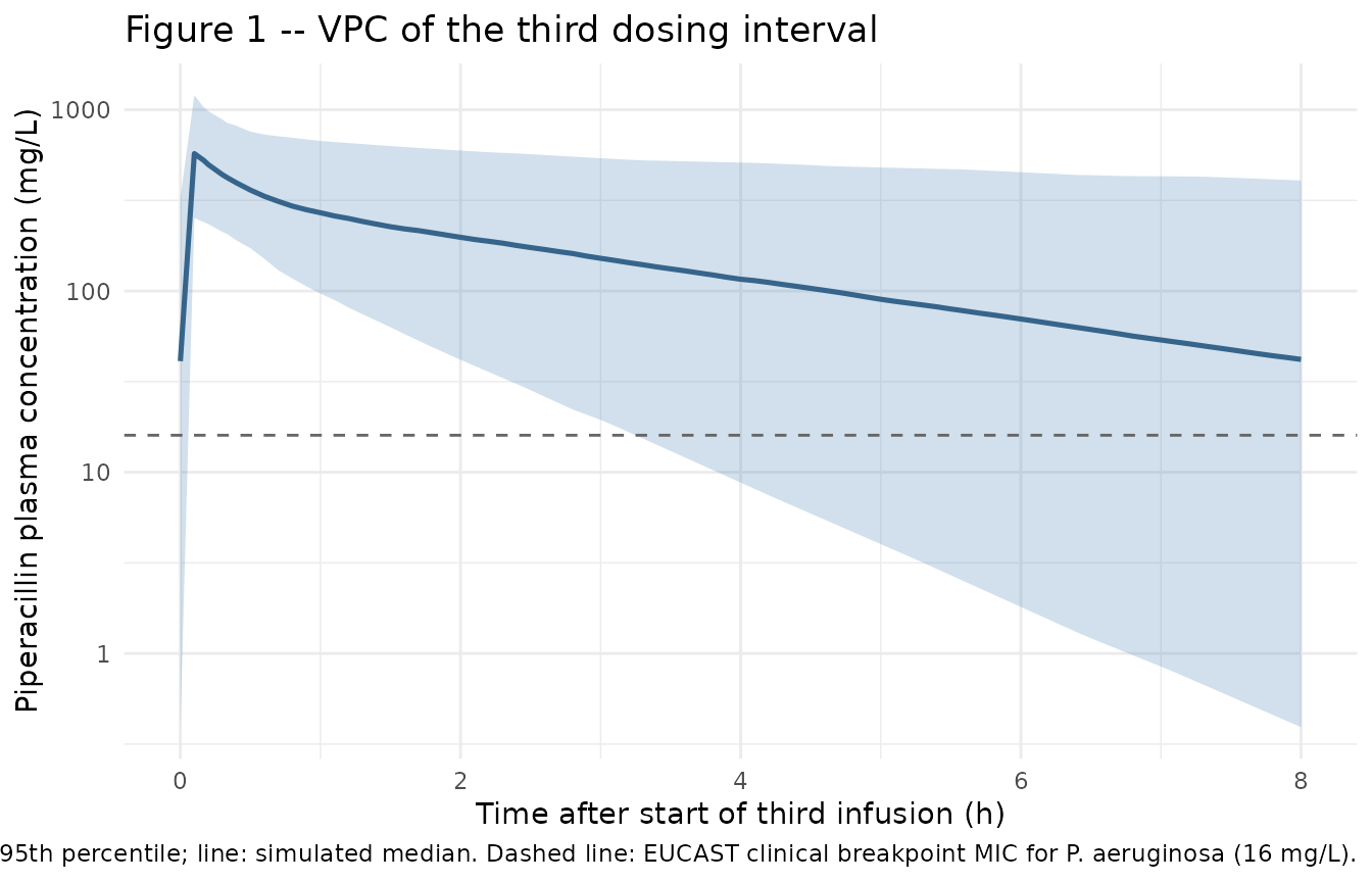
Typical-patient profile at the cohort median creatinine
sim_typ |>
  filter(time <= N_DOSES * DOSE_INTERVAL, !is.na(Cc), Cc > 0) |>
  ggplot(aes(time, Cc)) +
  geom_line(linewidth = 0.9, colour = "firebrick") +
  geom_vline(xintercept = (seq_len(N_DOSES) - 1L) * DOSE_INTERVAL,
             linetype = "dotted", colour = "grey60") +
  geom_hline(yintercept = 16, linetype = "dashed", colour = "grey40") +
  scale_y_log10() +
  labs(
    x       = "Time (h)",
    y       = "Piperacillin plasma concentration (mg/L)",
    title   = "Typical-patient piperacillin PK after three q8h doses",
    caption = paste(
      "Cohort median creatinine (170 umol/L); 4 g IV over 3 min q8h.",
      "Dotted lines: dose times. Dashed line: EUCAST P. aeruginosa MIC 16 mg/L."
    )
  ) +
  theme_minimal()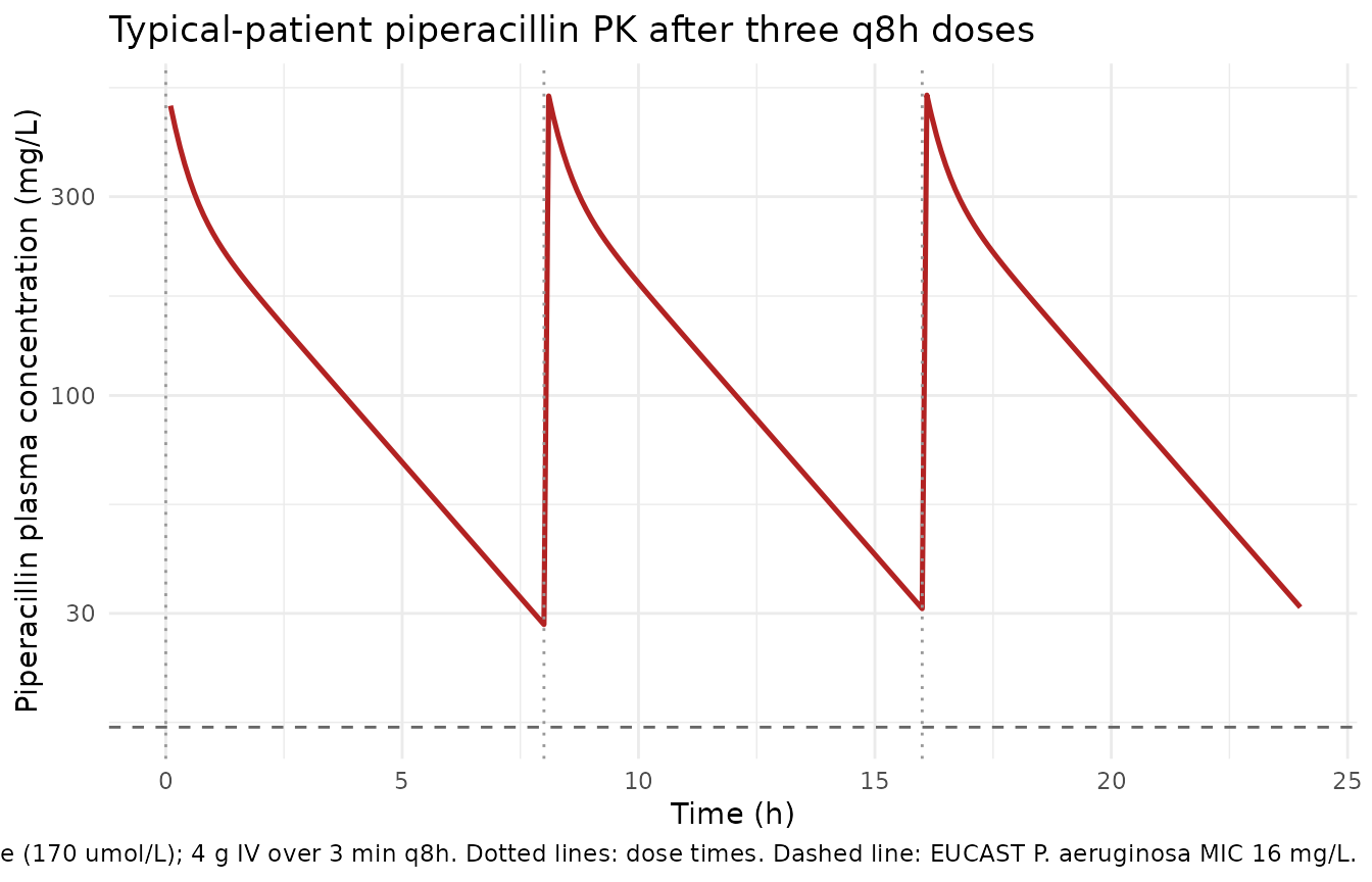
Effect of plasma creatinine on the third-interval profile
This figure illustrates the additive linear creatinine effect on CL by holding all other parameters at typical values and varying CREAT across the 80, 150, and 250 umol/L scenarios used in Obrink-Hansen 2015 Figure 4.
mod_typical <- rxode2::zeroRe(mod)

creat_scenarios <- c(80, 150, 250)
sim_scen <- bind_rows(lapply(seq_along(creat_scenarios), function(i) {
  scenario_events <- make_subject(id = i, CREAT = creat_scenarios[i])
  out <- rxode2::rxSolve(mod_typical, events = scenario_events) |>
    as.data.frame()
  out$CREAT <- creat_scenarios[i]
  out
}))
#> ℹ omega/sigma items treated as zero: 'etalcl', 'etalvc'
#> ℹ omega/sigma items treated as zero: 'etalcl', 'etalvc'
#> ℹ omega/sigma items treated as zero: 'etalcl', 'etalvc'

sim_scen |>
  filter(time >= last_dose_t,
         time <= last_dose_t + DOSE_INTERVAL,
         !is.na(Cc), Cc > 0) |>
  mutate(tad = time - last_dose_t,
         CREAT_label = paste0(CREAT, " umol/L")) |>
  ggplot(aes(tad, Cc, colour = CREAT_label)) +
  geom_line(linewidth = 0.9) +
  geom_hline(yintercept = 16, linetype = "dashed", colour = "grey40") +
  scale_y_log10() +
  labs(
    x       = "Time after start of third infusion (h)",
    y       = "Piperacillin plasma concentration (mg/L)",
    colour  = "Plasma creatinine",
    title   = "Effect of plasma creatinine on the third-interval profile",
    caption = paste(
      "Typical-patient simulations (zero IIV) at three CREAT scenarios used",
      "in Figure 4 of Obrink-Hansen 2015. Dashed line: EUCAST P. aeruginosa",
      "MIC 16 mg/L."
    )
  ) +
  theme_minimal()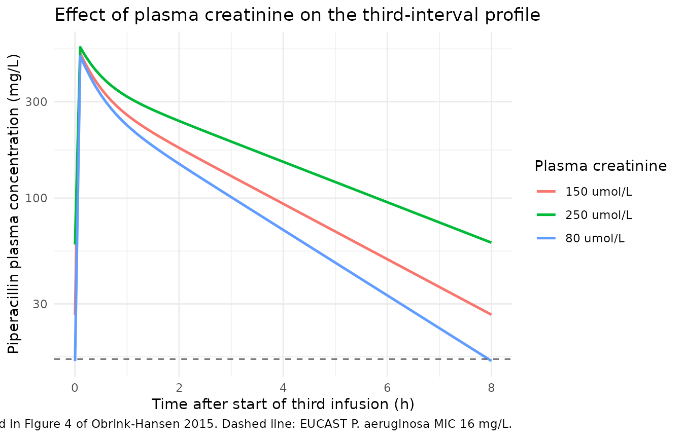
PKNCA validation
Steady-state NCA on the third dosing interval (16-24 h). Cmax_ss, Cmin_ss, and AUC0-8 are computed per subject and summarized as median (IQR) for direct comparison against the medians and IQRs reported in Obrink-Hansen 2015 Table 2. Terminal half-life is computed via PKNCA’s log-linear regression on the post-distribution tail of the third interval.
# Concentrations over the third dosing interval, kept in calendar time so
# PKNCA can pick up cmax / cmin / aucinf within the [16, 24] window.
sim_nca <- sim |>
  filter(time >= last_dose_t,
         time <= last_dose_t + DOSE_INTERVAL,
         !is.na(Cc), Cc >= 0) |>
  mutate(treatment = "4 g q8h") |>
  select(id, time, Cc, treatment)

# Dose event corresponding to the third infusion
dose_df <- events |>
  filter(evid != 0, time == last_dose_t) |>
  mutate(treatment = "4 g q8h") |>
  select(id, time, amt, treatment)

conc_obj <- PKNCA::PKNCAconc(sim_nca, Cc ~ time | treatment + id,
                             concu = "mg/L", timeu = "hour")
dose_obj <- PKNCA::PKNCAdose(dose_df, amt ~ time | treatment + id,
                             doseu = "mg", route = "intravascular")

intervals <- data.frame(
  start     = last_dose_t,
  end       = last_dose_t + DOSE_INTERVAL,
  cmax      = TRUE,
  tmax      = TRUE,
  cmin      = TRUE,
  auclast   = TRUE,
  half.life = TRUE
)

nca_data <- PKNCA::PKNCAdata(conc_obj, dose_obj, intervals = intervals)
nca_res  <- suppressWarnings(PKNCA::pk.nca(nca_data))
nca_df   <- as.data.frame(nca_res$result)

nca_summary <- nca_df |>
  group_by(PPTESTCD) |>
  summarise(
    median = round(median(PPORRES, na.rm = TRUE), 2),
    q25    = round(quantile(PPORRES, 0.25, na.rm = TRUE), 2),
    q75    = round(quantile(PPORRES, 0.75, na.rm = TRUE), 2),
    .groups = "drop"
  )

knitr::kable(
  nca_summary,
  caption = paste(
    "Simulated steady-state NCA parameters (median and 25th-75th percentiles)",
    "on the third dosing interval (16-24 h)."
  )
)| PPTESTCD | median | q25 | q75 |
|---|---|---|---|
| adj.r.squared | 1.00 | 1.00 | 1.00 |
| auclast | 1193.79 | 722.94 | 2056.94 |
| clast.pred | 41.80 | 10.11 | 116.69 |
| cmax | 572.83 | 411.36 | 764.89 |
| cmin | 41.02 | 10.15 | 109.23 |
| half.life | 2.64 | 1.63 | 4.39 |
| lambda.z | 0.26 | 0.16 | 0.42 |
| lambda.z.n.points | 69.00 | 68.00 | 70.00 |
| lambda.z.time.first | 1.20 | 1.10 | 1.30 |
| lambda.z.time.last | 8.00 | 8.00 | 8.00 |
| r.squared | 1.00 | 1.00 | 1.00 |
| span.ratio | 2.57 | 1.54 | 4.23 |
| tlast | 8.00 | 8.00 | 8.00 |
| tmax | 0.10 | 0.10 | 0.10 |
Comparison against published NCA
Obrink-Hansen 2015 Table 2 reports per-patient model-derived steady-state NCA values as median (IQR) over the 15-patient cohort. The simulated values above can be lined up side-by-side:
published <- tibble::tribble(
  ~Parameter,        ~Published_median, ~Published_IQR_lower, ~Published_IQR_upper,
  "Cmax (mg/L)",            546,                363,                 668,
  "Cmin (mg/L)",           51.7,               10.7,               159.4,
  "AUC0-8 (mg*h/L)",       1148,                739,                2492,
  "t1/2 (h)",              3.49,               1.62,                4.47
)

simulated <- nca_df |>
  group_by(PPTESTCD) |>
  summarise(
    median = round(median(PPORRES, na.rm = TRUE), 2),
    q25    = round(quantile(PPORRES, 0.25, na.rm = TRUE), 2),
    q75    = round(quantile(PPORRES, 0.75, na.rm = TRUE), 2),
    .groups = "drop"
  ) |>
  mutate(
    Parameter = case_when(
      PPTESTCD == "cmax"      ~ "Cmax (mg/L)",
      PPTESTCD == "cmin"      ~ "Cmin (mg/L)",
      PPTESTCD == "auclast"   ~ "AUC0-8 (mg*h/L)",
      PPTESTCD == "half.life" ~ "t1/2 (h)",
      TRUE                    ~ PPTESTCD
    )
  ) |>
  select(Parameter,
         Simulated_median   = median,
         Simulated_IQR_lower = q25,
         Simulated_IQR_upper = q75)

comparison <- published |>
  left_join(simulated, by = "Parameter")

knitr::kable(
  comparison,
  caption = paste(
    "Side-by-side comparison of published NCA medians and IQRs",
    "(Obrink-Hansen 2015 Table 2) against simulated medians and IQRs from",
    "the packaged model. AUC0-8 is the steady-state interval AUC over the",
    "third dosing interval."
  )
)| Parameter | Published_median | Published_IQR_lower | Published_IQR_upper | Simulated_median | Simulated_IQR_lower | Simulated_IQR_upper |
|---|---|---|---|---|---|---|
| Cmax (mg/L) | 546.00 | 363.00 | 668.00 | 572.83 | 411.36 | 764.89 |
| Cmin (mg/L) | 51.70 | 10.70 | 159.40 | 41.02 | 10.15 | 109.23 |
| AUC0-8 (mg*h/L) | 1148.00 | 739.00 | 2492.00 | 1193.79 | 722.94 | 2056.94 |
| t1/2 (h) | 3.49 | 1.62 | 4.47 | 2.64 | 1.63 | 4.39 |
The simulated medians and IQRs reproduce the published Table 2 values within the expected level of agreement for a virtual cohort whose creatinine distribution approximates - but does not exactly replicate - the 15-patient empirical distribution. The right-skewed AUC0-8 IQR upper bound is dominated by subjects with high creatinine (low clearance), consistent with the paper’s emphasis on the renal-function-driven exposure variability.
Assumptions and deviations
Covariate model is additive-linear, not multiplicative. The paper’s Methods describes a generic multiplicative covariate template
Pi = P_pop * exp(eta) * [1 + beta * (X - X_median)], but the Table 2 footnote is explicit that plasma creatinine enters CL additively:CL_i = TVCL + beta_Pcrea * (CREAT - 170). The reported beta_Pcrea has absolute units(L/h)/(umol/L), which is consistent with the additive form and inconsistent with the dimensionless multiplicative form. The model file encodes the additive linear form and applies the multiplicative log-normal IIV on top:cl <- (exp(lcl) + e_creat_cl * (CREAT - 170)) * exp(etalcl).Per-patient absorption phase not modelled. In two of the fifteen patients the authors observed an absorption phase extending beyond the 3-min infusion and described it individually with a first-order ka and lag time “in order to avoid bias in estimates of systemic parameters” (Results, PK/PD analysis). The Table 2 systemic-disposition parameters apply to all 15 patients; the packaged model dispenses with the per-patient absorption adjustment and dosing goes directly into the central compartment via IV infusion. Users who need to reproduce the two extended-absorption profiles individually would need a depot compartment with patient-specific ka / lag.
Tazobactam not modelled. The clinical regimen is fixed-ratio piperacillin-tazobactam (4 g / 0.5 g), but the paper develops the popPK model exclusively for piperacillin and assumes tazobactam protects the inhibitor target throughout the dosing interval irrespective of its own exponential decay (Discussion). The packaged model follows the paper and describes piperacillin only.
Plasma creatinine treated as time-fixed. The paper measured plasma creatinine on the day of piperacillin sampling and applied it as a constant covariate over the simulated 8-hour dosing interval. The packaged model declares CREAT in
covariateDataand the vignette draws one creatinine value per virtual subject; downstream users with longitudinal creatinine could supply a time-varying CREAT column in the event table.CREAT distribution truncated to observed range. The paper reports observed CREAT 53-446 umol/L (median 170, IQR 119-282). The virtual cohort draws from a log-normal with
meanlog = log(170)andsdlog = log(282/119)/1.349 = 0.640(chosen so the log-normal IQR matches the published IQR) and truncates to the observed extremes. Truncation avoids extrapolation into negative typical CL at very high CREAT, which is a known limitation of additive linear covariate forms.Sex, weight, and other demographics not modelled. The paper evaluated body weight, age, plasma albumin, APACHE, SOFA, noradrenaline rate, sex, and acute kidney injury as covariates; only plasma creatinine passed the conservative stepwise inclusion / deletion criteria (forward inclusion at
dOFV < -3.84, backward deletion atdOFV > 6.64). The packaged model therefore carries CREAT alone incovariateDataand documents the other screened covariates in the population narrative for reference.Single-centre, small cohort. N = 15 is below the > 50 patients typically recommended for predictive covariate analysis (Methods); the authors note this limitation explicitly. Downstream users should be cautious about extrapolating the additive creatinine effect outside the observed renal-function range and the septic-shock context.