Iloperidone and metabolites M1 (P-88) and M2 (P-95) (Pei 2016)
Source:vignettes/articles/Pei_2016_iloperidone.Rmd
Pei_2016_iloperidone.RmdModel and source
- Citation: Pei Q, Huang L, Huang J, Gu J-K, Kuang Y, Zuo X-C, Ding J-J, Tan H-Y, Guo C-X, Liu S-K, Yang G-P (2016). Influences of CYP2D610 polymorphisms on the pharmacokinetics of iloperidone and its metabolites in Chinese patients with schizophrenia: a population pharmacokinetic analysis. Acta Pharmacologica Sinica* 37(11):1499-1508. doi:10.1038/aps.2016.96.
- Article: https://doi.org/10.1038/aps.2016.96
The package model can be loaded with:
mod_fn <- readModelDb("Pei_2016_iloperidone")
mod    <- rxode2::rxode2(mod_fn())
Population
Pei 2016 enrolled 70 Chinese patients (28 male, 42 female; mean age 34 +/- 12 years; mean weight 62.2 +/- 10.5 kg) with schizophrenia or schizoaffective disorder (DSM-IV) at 13 hospitals in China. The doses were titrated from 2 mg/day on day 1 up to 12 mg/day on day 4 (twice daily), then individually adjusted on days 5-14 according to patient tolerance, and maintained at a fixed dose (12, 16, 20, or 24 mg/day) on days 15-28. Plasma iloperidone, M1 (P-88), and M2 (P-95) were measured at four sparse sampling time points: C15-0 (predose day 15, the first day of fixed-dose maintenance), C28-0 (predose day 28), C28-4 (4 h post-AM-dose day 28), and C28-12 (12 h post-AM-dose day 28). The cohort yielded 804 concentration measurements across the three analytes (266 iloperidone, 268 M1, 270 M2). CYP2D610 (rs1065852) genotype distribution: C/C 11/70 (15.7%), C/T 42/70 (60.0%), T/T 17/70 (24.3%) – consistent with the 48-70% 10 allele frequency reported for Chinese populations.
The full population metadata are available programmatically via
readModelDb("Pei_2016_iloperidone")$population.
Source trace
Every parameter and equation traces back to the Pei 2016 Table 3
final parameter estimates, Methods ‘Population pharmacokinetic (PPK)
modeling’, and the Results ‘Population pharmacokinetic (PPK) models’
equations. Per-parameter source locations are also recorded inline next
to each ini() entry in
inst/modeldb/specificDrugs/Pei_2016_iloperidone.R.
| Equation / parameter | Value | Source location |
|---|---|---|
lka = fixed(log(2.26)) (Ka, 1/h; FIXED) |
2.26 | Table 3 Ka (FIX); Methods (Ka estimated from healthy-volunteer digitisation and fixed) |
lkel = log(0.067) (K20, 1/h) |
0.067 | Table 3 K20 (RSE 13.3%; bootstrap 95% CI 0.051-0.082) |
lkel_form_p88 = log(0.00451) (K23, 1/h) |
0.00451 | Table 3 K23 (RSE 27.7%; bootstrap 95% CI 0.00276-0.00627) |
lkel_form_p95 = log(0.00649) (K24, 1/h) |
0.00649 | Table 3 K24 (RSE 31.1%; bootstrap 95% CI 0.00292-0.0113) |
lkel_p88 = log(0.160) (K30, 1/h) |
0.160 | Table 3 K30 (RSE 30.6%; bootstrap 95% CI 0.101-0.223) |
lkel_p95 = log(0.106) (K40, 1/h) |
0.106 | Table 3 K40 (RSE 29.6%; bootstrap 95% CI 0.057-0.173) |
lvc = log(679) (V2, L) |
679 | Table 3 V2 (RSE 13.4%; bootstrap 95% CI 495-979) |
lvc_p88 = fixed(log(10)) (V3, L; FIXED) |
10 | Table 3 V3 (FIX); Methods (no conversion-fraction identifiability) |
lvc_p95 = fixed(log(10)) (V4, L; FIXED) |
10 | Table 3 V4 (FIX); Methods (no conversion-fraction identifiability) |
e_cyp2d6_star10_hom_kel_form_p88 = log(1.34) (T/T on
K23) |
1.34 | Table 3 CYP2D6*10 T/T on K23 (RSE 12.4%; bootstrap 95% CI 1.15-1.55) |
e_cyp2d6_star10_het_kel_form_p95 = log(0.693) (C/T on
K24) |
0.693 | Table 3 CYP2D6*10 C/T on K24 (RSE 18.9%; bootstrap 95% CI 0.518-0.919) |
e_cyp2d6_star10_hom_kel_form_p95 = log(0.492) (T/T on
K24) |
0.492 | Table 3 CYP2D6*10 T/T on K24 (RSE 24.2%; bootstrap 95% CI 0.362-0.652) |
etalkel ~ log(1 + 0.195^2) (BSV on K20) |
19.5% CV | Table 3 BSV K20 (RSE 34%; bootstrap 95% CI 6.7-29.8%) |
etalvc ~ log(1 + 0.358^2) (BSV on V2) |
35.8% CV | Table 3 BSV V2 (RSE 19%; bootstrap 95% CI 25.6-45.6%) |
etalkel_form_p88 ~ log(1 + 0.196^2) (BSV on K23) |
19.6% CV | Table 3 BSV K23 (RSE 26%; bootstrap 95% CI 8.5-28.1%) |
etalkel_form_p95 ~ log(1 + 0.409^2) (BSV on K24) |
40.9% CV | Table 3 BSV K24 (RSE 13%; bootstrap 95% CI 30.5-48.2%) |
propSd = 0.377 (proportional, iloperidone) |
37.7% CV | Table 3 CV1 (RSE 15%; bootstrap 95% CI 32.8-42.6%) |
propSd_p88 = 0.236 (proportional, M1) |
23.6% CV | Table 3 CV2 (RSE 9%; bootstrap 95% CI 19.1-29.0%) |
propSd_p95 = 0.221 (proportional, M2) |
22.1% CV | Table 3 CV3 (RSE 7%; bootstrap 95% CI 17.2-26.5%) |
| 1-compartment first-order absorption + parallel-pathway parent elimination | – | Methods ‘Population pharmacokinetic (PPK) modeling’; Figure 1 (model schematic) |
| Two metabolite compartments with own first-order elimination | – | Figure 1 (model schematic); Results ‘Population pharmacokinetic (PPK) models’ |
| Mass-unit (not molar) flow from parent to metabolites | – | Methods ‘Population pharmacokinetic (PPK) modeling’ (MW iloperidone 427.3, M1 429.4, M2 429.2 g/mol, within 0.5%) |
| V3 = V4 = 10 L (FIXED apparent metabolite volumes) | – | Methods ‘Population pharmacokinetic (PPK) modeling’ (no conversion-fraction identifiability without tracer) |
| IOV on K20 (27.3% CV) reported but not encoded | – | Table 3 IOV K20; see Assumptions and deviations below |
Virtual cohort
The virtual cohort approximates the Pei 2016 study design. Body
weight is drawn from a truncated-normal approximation of the Table 1
cohort summary (mean 62.2 kg, SD 10.5, truncated to 40-100 kg).
CYP2D6*10 genotype is assigned via multinomial sampling with the
observed frequencies from Table 1 (C/C 15.7%, C/T 60.0%, T/T 24.3%). The
two binary indicators CYP2D6_STAR10_HET and
CYP2D6_STAR10_HOM are derived from the assigned genotype
(C/C wild-type is the implicit reference: both indicators = 0). Sample
size is set to 200 (about 3x the source cohort) to stabilise the
simulated VPC percentiles across the three genotype strata.
set.seed(20260603L)
n_sub <- 200L

geno_levels <- c("C/C", "C/T", "T/T")
geno_probs  <- c(0.157, 0.600, 0.243)

subjects <- data.frame(
  id        = seq_len(n_sub),
  WT        = round(pmin(pmax(rnorm(n_sub, mean = 62.2, sd = 10.5), 40), 100), 1),
  genotype  = sample(geno_levels, n_sub, replace = TRUE, prob = geno_probs)
)
subjects$CYP2D6_STAR10_HET <- as.integer(subjects$genotype == "C/T")
subjects$CYP2D6_STAR10_HOM <- as.integer(subjects$genotype == "T/T")
subjects$treatment         <- subjects$genotype

table(subjects$genotype)
#>
#> C/C C/T T/T
#>  30 118  52
Maintenance dosing: the source study used 12, 16, 20, or 24 mg/day given twice daily for days 15-28 of stable-dose maintenance. For the simulation, each virtual subject receives 8 mg of oral iloperidone twice daily (every 12 h) – equivalent to 16 mg/day, the second-most-frequent dose level (12/70 = 17%) and a representative midpoint of the cohort’s titrated maintenance dose range. The simulation runs for 14 days (28 doses), with dense observations over the final dosing interval to support both VPC display and PKNCA at steady state, plus per-sampling-time observations matching the four published time points C15-0, C28-0, C28-4, C28-12.
dose_amt    <- 8           # mg per dose (16 mg/day q12h)
n_days      <- 14L
dose_times  <- seq(0, by = 12, length.out = 2 * n_days)
obs_start   <- max(dose_times)  # time of the last dose
obs_times   <- sort(unique(c(
  obs_start + seq(0, 12, by = 0.25),
  # Source sampling time points relative to the final dose (treat day 15 = day 14 + 12 h):
  obs_start - 12,         # C15-0 (predose 12 h before final dose; approximates day-15 trough)
  obs_start,              # C28-0 (predose immediately before final dose)
  obs_start + 4,          # C28-4 (4 h post final dose)
  obs_start + 12          # C28-12 (12 h post final dose)
)))

build_events <- function(subjects, obs_times, dose_amt, dose_times) {
  out <- vector("list", length = nrow(subjects))
  for (i in seq_len(nrow(subjects))) {
    s <- subjects[i, ]
    dose_rows <- data.frame(
      id                 = s$id,
      time               = dose_times,
      evid               = 1L,
      amt                = dose_amt,
      cmt                = "depot",
      WT                 = s$WT,
      CYP2D6_STAR10_HET  = s$CYP2D6_STAR10_HET,
      CYP2D6_STAR10_HOM  = s$CYP2D6_STAR10_HOM,
      treatment          = s$treatment
    )
    obs_rows <- data.frame(
      id                 = s$id,
      time               = obs_times,
      evid               = 0L,
      amt                = 0,
      cmt                = "Cc",
      WT                 = s$WT,
      CYP2D6_STAR10_HET  = s$CYP2D6_STAR10_HET,
      CYP2D6_STAR10_HOM  = s$CYP2D6_STAR10_HOM,
      treatment          = s$treatment
    )
    out[[i]] <- rbind(dose_rows, obs_rows)
  }
  ev <- dplyr::bind_rows(out)
  ev[order(ev$id, ev$time, -ev$evid), ]
}

events <- build_events(subjects, obs_times, dose_amt, dose_times)
Simulation
Stochastic simulation carrying IIV on K20 (lkel), V2
(lvc), K23 (lkel_form_p88), and K24
(lkel_form_p95). Ka is fixed and has no IIV; K30, K40, V3,
V4 are also estimated or fixed without IIV per the source.
sim <- rxode2::rxSolve(
mod,
events = events,
keep = c("WT", "CYP2D6_STAR10_HET", "CYP2D6_STAR10_HOM", "treatment")
) |>
as.data.frame()
sim_ss <- sim |>
dplyr::mutate(tad = time - obs_start) |>
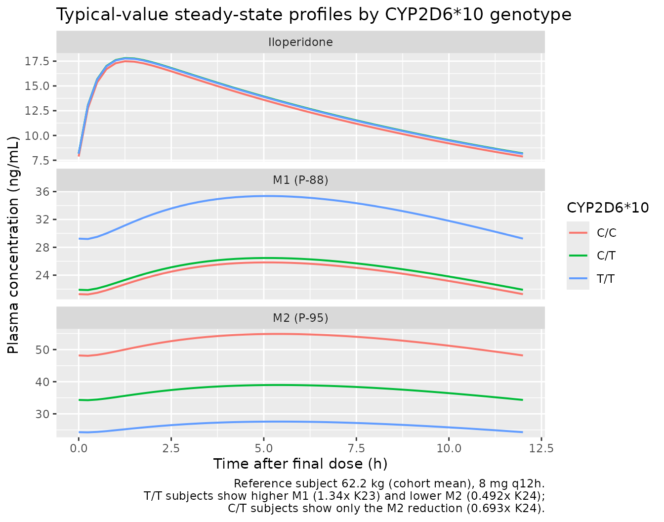
dplyr::filter(tad >= 0, tad <= 12)A typical-value (no-IIV, no-residual) replication for each of the three CYP2D6*10 genotypes at the cohort mean weight, useful for narrative comparison against the paper’s reported point estimates.
mod_typical <- rxode2::zeroRe(mod)

typical_subjects <- data.frame(
  id                = 1:3,
  WT                = 62.2,
  genotype          = c("C/C", "C/T", "T/T"),
  CYP2D6_STAR10_HET = c(0L, 1L, 0L),
  CYP2D6_STAR10_HOM = c(0L, 0L, 1L),
  treatment         = c("C/C", "C/T", "T/T")
)

typical_events <- build_events(typical_subjects, obs_times, dose_amt, dose_times)
sim_typ <- rxode2::rxSolve(
  mod_typical,
  events = typical_events,
  keep   = c("WT", "CYP2D6_STAR10_HET", "CYP2D6_STAR10_HOM", "treatment")
) |>
  as.data.frame() |>
  dplyr::mutate(tad = time - obs_start) |>
  dplyr::filter(tad >= 0, tad <= 12)
#> ℹ omega/sigma items treated as zero: 'etalkel', 'etalvc', 'etalkel_form_p88', 'etalkel_form_p95'
#> Warning: multi-subject simulation without without 'omega'
Replicate published figures
Figure 2: C/D ratios at the four sampling time points, stratified by CYP2D6*10 genotype
Pei 2016 Figure 2 shows concentration / daily-dose ratios (C/D) for iloperidone, M1, and M2 at the four sampling time points, stratified by CYP2D6*10 genotype (C/C, C/T, T/T). The package model reproduces the qualitative patterns reported in the paper:
- Iloperidone C/D is similar across genotypes at most time points but slightly differs at C28-12 (per the paper’s statistical test). The mechanistic basis is that the total iloperidone elimination rate (K20 + K23 + K24) is nearly identical across genotypes (~0.076-0.078 1/h): T/T subjects’ lower K24 is approximately offset by their higher K23, so apparent oral clearance of the parent is not strongly genotype-dependent (Pei 2016 Discussion).
- M1 C/D is higher in T/T than C/C or C/T at C28-0, C28-4, C28-12 (T/T has 1.34-fold higher K23 -> more iloperidone is converted to M1).
- M2 C/D is lower in C/T (0.693x) and T/T (0.492x) than C/C at C15-0 and C28-0 (reduced CYP2D6 activity in *10-allele carriers -> less M2 formation).
The simulation reports C/D in (ng/mL) / (mg/day); the source paper uses a similar unit (their y-axis is “C/D” without explicit units, but the value ranges and the table-reported plasma concentrations both confirm ng/mL relative to mg).
daily_dose <- 2 * dose_amt  # 16 mg/day

# C/D ratios at the four published time points (relative to the final dose at obs_start):
sampling_times <- c(
  `C15-0`  = obs_start - 12,
  `C28-0`  = obs_start,
  `C28-4`  = obs_start + 4,
  `C28-12` = obs_start + 12
)

cd_ratios <- sim |>
  dplyr::filter(round(time, 2) %in% round(sampling_times, 2)) |>
  dplyr::mutate(
    sample_label = factor(
      sapply(time, function(t) names(sampling_times)[which.min(abs(sampling_times - t))]),
      levels = c("C15-0", "C28-0", "C28-4", "C28-12")
    )
  ) |>
  dplyr::transmute(
    id, treatment, sample_label,
    Iloperidone = Cc / daily_dose,
    M1_P88      = Cc_p88 / daily_dose,
    M2_P95      = Cc_p95 / daily_dose
  ) |>
  tidyr::pivot_longer(c(Iloperidone, M1_P88, M2_P95),
                      names_to = "analyte", values_to = "cd_ratio")

cd_ratios |>
  ggplot(aes(treatment, cd_ratio, fill = treatment)) +
  geom_boxplot(outlier.size = 0.5, alpha = 0.6) +
  facet_grid(analyte ~ sample_label, scales = "free_y") +
  labs(x = "CYP2D6*10 genotype", y = "C/D ratio  ((ng/mL) / (mg/day))",
       fill = "CYP2D6*10",
       title = "C/D ratios at the four published sampling time points",
       caption = paste(
         "Replicates Figure 2 of Pei 2016 (boxplots of C/D by CYP2D6*10 genotype).",
         "Daily dose 16 mg/day; CYP2D6*10 effects on K23, K24 drive the metabolite shifts."
       )) +
  theme(legend.position = "none")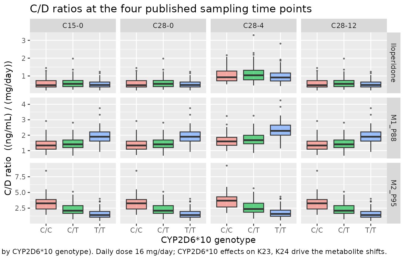
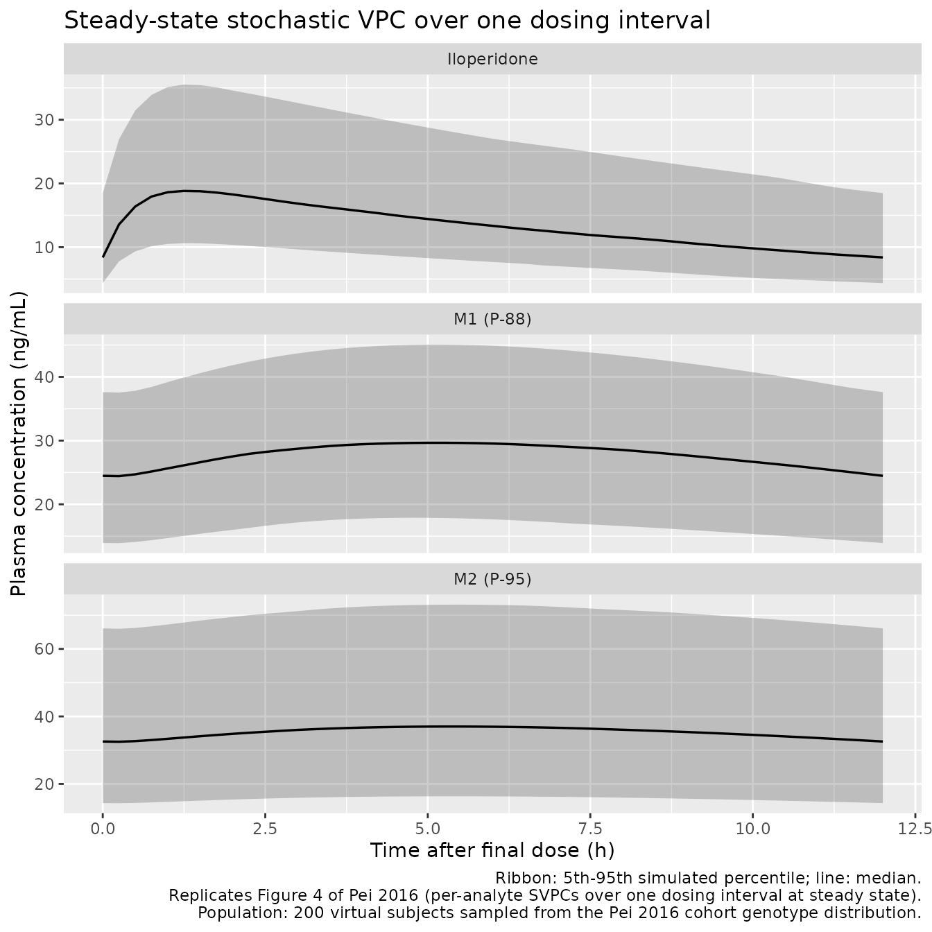
Figure 4-style: stochastic VPC over one dosing interval at steady state
Pei 2016 Figure 4 shows the SVPC (Standard Visual Predictive Check) plots for iloperidone, M1, and M2 against time, with the simulated 5th, 50th, and 95th percentile bands. The package model reproduces the per-analyte time courses over a single dosing interval at steady state.
vpc_data <- sim_ss |>
  dplyr::select(tad, treatment, Cc, Cc_p88, Cc_p95) |>
  tidyr::pivot_longer(c(Cc, Cc_p88, Cc_p95), names_to = "analyte", values_to = "conc") |>
  dplyr::mutate(
    analyte = dplyr::recode(analyte,
                            Cc     = "Iloperidone",
                            Cc_p88 = "M1 (P-88)",
                            Cc_p95 = "M2 (P-95)"),
    analyte = factor(analyte, levels = c("Iloperidone", "M1 (P-88)", "M2 (P-95)"))
  )

vpc_data |>
  dplyr::group_by(analyte, tad) |>
  dplyr::summarise(
    p05 = quantile(conc, 0.05, na.rm = TRUE),
    p50 = quantile(conc, 0.50, na.rm = TRUE),
    p95 = quantile(conc, 0.95, na.rm = TRUE),
    .groups = "drop"
  ) |>
  ggplot(aes(tad, p50)) +
  geom_ribbon(aes(ymin = p05, ymax = p95), alpha = 0.25) +
  geom_line(linewidth = 0.6) +
  facet_wrap(~ analyte, ncol = 1, scales = "free_y") +
  labs(x = "Time after final dose (h)",
       y = "Plasma concentration (ng/mL)",
       title = "Steady-state stochastic VPC over one dosing interval",
       caption = paste(
         "Ribbon: 5th-95th simulated percentile; line: median.",
         "Replicates Figure 4 of Pei 2016 (per-analyte SVPCs over one dosing interval at steady state).",
         "Population: 200 virtual subjects sampled from the Pei 2016 cohort genotype distribution.",
         sep = "\n"
       ))
Typical-value concentration profiles by genotype
sim_typ |>
  dplyr::select(tad, treatment, Iloperidone = Cc, `M1 (P-88)` = Cc_p88, `M2 (P-95)` = Cc_p95) |>
  tidyr::pivot_longer(c(Iloperidone, `M1 (P-88)`, `M2 (P-95)`),
                      names_to = "analyte", values_to = "conc") |>
  dplyr::mutate(
    analyte = factor(analyte, levels = c("Iloperidone", "M1 (P-88)", "M2 (P-95)"))
  ) |>
  dplyr::filter(conc > 0) |>
  ggplot(aes(tad, conc, colour = treatment)) +
  geom_line(linewidth = 0.7) +
  facet_wrap(~ analyte, ncol = 1, scales = "free_y") +
  labs(x = "Time after final dose (h)",
       y = "Plasma concentration (ng/mL)",
       colour = "CYP2D6*10",
       title = "Typical-value steady-state profiles by CYP2D6*10 genotype",
       caption = paste(
         "Reference subject 62.2 kg (cohort mean), 8 mg q12h.",
         "T/T subjects show higher M1 (1.34x K23) and lower M2 (0.492x K24);",
         "C/T subjects show only the M2 reduction (0.693x K24).",
         sep = "\n"
       ))
PKNCA validation
Steady-state NCA over the final dosing interval (0-12 h post final dose), stratified by CYP2D6*10 genotype and by analyte. Cmax, Tmax, and AUC0-tau (12 h) are computed for each combination so the impact of the genotype-specific K23 and K24 effects on metabolite exposure is visible directly.
nca_long <- sim_ss |>
  dplyr::select(id, tad, Cc, Cc_p88, Cc_p95, treatment) |>
  tidyr::pivot_longer(c(Cc, Cc_p88, Cc_p95),
                      names_to = "analyte", values_to = "conc") |>
  dplyr::mutate(analyte = dplyr::recode(analyte,
                                        Cc     = "iloperidone",
                                        Cc_p88 = "M1_P88",
                                        Cc_p95 = "M2_P95")) |>
  dplyr::filter(!is.na(conc))

conc_obj <- PKNCA::PKNCAconc(
  nca_long,
  conc ~ tad | analyte + treatment / id,
  concu = "ng/mL", timeu = "h"
)

# Only the parent has a dose record; PKNCA accepts a single-analyte dose
# object that gets matched to the iloperidone concentration block.
dose_df <- data.frame(
  id        = subjects$id,
  time      = 0,
  amt       = dose_amt,
  analyte   = "iloperidone",
  treatment = subjects$treatment
)
dose_obj <- PKNCA::PKNCAdose(
  dose_df,
  amt ~ time | analyte + treatment + id,
  doseu = "mg"
)

intervals <- data.frame(
  start    = 0,
  end      = 12,
  cmax     = TRUE,
  tmax     = TRUE,
  auclast  = TRUE,
  cmin     = TRUE
)

nca_res <- PKNCA::pk.nca(
  PKNCA::PKNCAdata(conc_obj, dose_obj, intervals = intervals)
)
summarise_nca <- function(res) {
  df <- as.data.frame(res$result)
  df |>
    dplyr::filter(PPTESTCD %in% c("cmax", "tmax", "auclast", "cmin")) |>
    dplyr::group_by(analyte, treatment, PPTESTCD) |>
    dplyr::summarise(
      median = median(PPORRES, na.rm = TRUE),
      p05    = quantile(PPORRES, 0.05, na.rm = TRUE),
      p95    = quantile(PPORRES, 0.95, na.rm = TRUE),
      .groups = "drop"
    )
}

nca_summary <- summarise_nca(nca_res) |>
  dplyr::arrange(analyte, treatment, PPTESTCD)

knitr::kable(nca_summary,
             caption = paste(
               "Simulated steady-state NCA over the 0-12 h dosing interval after the",
               "final dose, stratified by CYP2D6*10 genotype and analyte.",
               "Cmax / Cmin in ng/mL, Tmax in h, AUC0-tau in ng*h/mL.",
               "Median [5%-95%] across 200 simulated subjects."
             ),
digits = 3)| analyte | treatment | PPTESTCD | median | p05 | p95 |
|---|---|---|---|---|---|
| M1_P88 | C/C | auclast | 287.776 | 176.193 | 477.507 |
| M1_P88 | C/C | cmax | 25.742 | 15.969 | 42.207 |
| M1_P88 | C/C | cmin | 21.292 | 12.451 | 35.822 |
| M1_P88 | C/C | tmax | 5.000 | 4.862 | 5.250 |
| M1_P88 | C/T | auclast | 305.361 | 201.126 | 433.770 |
| M1_P88 | C/T | cmax | 27.031 | 18.064 | 37.789 |
| M1_P88 | C/T | cmin | 22.490 | 14.630 | 33.241 |
| M1_P88 | C/T | tmax | 5.000 | 5.000 | 5.250 |
| M1_P88 | T/T | auclast | 412.663 | 294.555 | 587.743 |
| M1_P88 | T/T | cmax | 36.775 | 26.276 | 52.199 |
| M1_P88 | T/T | cmin | 30.357 | 21.702 | 43.543 |
| M1_P88 | T/T | tmax | 5.000 | 5.000 | 5.250 |
| M2_P95 | C/C | auclast | 677.496 | 341.023 | 1091.183 |
| M2_P95 | C/C | cmax | 59.568 | 29.964 | 94.329 |
| M2_P95 | C/C | cmin | 52.122 | 25.823 | 85.160 |
| M2_P95 | C/C | tmax | 5.500 | 5.112 | 5.500 |
| M2_P95 | C/T | auclast | 435.185 | 238.692 | 837.302 |
| M2_P95 | C/T | cmax | 38.064 | 20.694 | 72.691 |
| M2_P95 | C/T | cmin | 33.382 | 18.548 | 64.426 |
| M2_P95 | C/T | tmax | 5.500 | 5.250 | 5.500 |
| M2_P95 | T/T | auclast | 292.990 | 140.090 | 691.903 |
| M2_P95 | T/T | cmax | 25.423 | 12.318 | 60.451 |
| M2_P95 | T/T | cmin | 22.342 | 10.593 | 52.943 |
| M2_P95 | T/T | tmax | 5.500 | 5.250 | 5.500 |
| iloperidone | C/C | auclast | 150.612 | 96.257 | 343.162 |
| iloperidone | C/C | cmax | 17.845 | 11.920 | 35.154 |
| iloperidone | C/C | cmin | 7.698 | 3.747 | 20.297 |
| iloperidone | C/C | tmax | 1.250 | 1.250 | 1.250 |
| iloperidone | C/T | auclast | 169.786 | 92.969 | 326.982 |
| iloperidone | C/T | cmax | 19.212 | 10.619 | 35.699 |
| iloperidone | C/T | cmin | 8.906 | 4.743 | 18.266 |
| iloperidone | C/T | tmax | 1.250 | 1.250 | 1.250 |
| iloperidone | T/T | auclast | 152.878 | 83.476 | 298.694 |
| iloperidone | T/T | cmax | 17.251 | 10.243 | 34.291 |
| iloperidone | T/T | cmin | 7.909 | 4.147 | 16.249 |
| iloperidone | T/T | tmax | 1.250 | 1.250 | 1.250 |
Comparison against the published expected pattern
Pei 2016 does not publish steady-state NCA values per se; the paper’s results focus on C/D ratios at the four sampling time points and on the OFV-driven covariate model selection (Table 2). The expected qualitative patterns from the source paper’s mechanism are:
| Quantity | C/C reference | C/T (HET) | T/T (HOM) | Source |
|---|---|---|---|---|
| K23 (M1 formation) | 0.00451 | 0.00451 | 0.00604 | Table 3 + CYP2D6*10 T/T = 1.34 |
| K24 (M2 formation) | 0.00649 | 0.00450 | 0.00319 | Table 3 + CYP2D6*10 C/T = 0.693, T/T = 0.492 |
| Total iloperidone elimination (K20 + K23 + K24) | 0.0780 | 0.0760 | 0.0762 | Sum of above plus K20 = 0.067 |
Because the total iloperidone elimination is nearly genotype-invariant, simulated iloperidone Cmax / AUCss should be similar across genotype strata (slight differences arise from the lognormal IIV mixing). M1 (P-88) AUCss should rise approximately 34% in T/T vs C/C + C/T; M2 (P-95) AUCss should fall approximately 31% in C/T and 51% in T/T vs C/C. The simulated PKNCA table above should reproduce these qualitative patterns within the per-stratum 5%-95% bands.
Assumptions and deviations
Inter-occasion variability on K20 (27.3% CV) not encoded as a separate eta. Pei 2016 Table 3 reports IOV on K20 in addition to the BSV (19.5% CV). The package model encodes the BSV via
etalkelbut does not carry IOV as a separate per-occasion random effect. A downstream user who needs occasion-aware simulation (e.g., to reproduce within-subject variability between days 15-0 and 28-0 in the same patient) should add an IOV eta via the rxode2 IOV mechanism (etalkel_iovwith a per-occasion design column). The deterministic typical-value trajectories and the BSV-driven 5%-95% percentile bands are unaffected by the omission.Ka FIXED at 2.26 1/h from a separate forward analysis. Pei 2016 estimated Ka in a two-step procedure: (1) a separate two-compartment fit of healthy-volunteer iloperidone concentration-time data digitised from ref [23] using Getdata Graph Digitizer, which yielded Ka = 1.68 1/h, and (2) fixed at 2.26 1/h for the patient model. The Methods section justifies the fixing because no Ka has been reported in the published literature for iloperidone in patients and the cohort’s sparse sampling (no early absorption phase observations) does not permit reliable in-study Ka estimation. The package model preserves this fix exactly. Users sensitive to absorption-phase predictions should be aware that Ka carries a non-trivial systematic uncertainty rooted in the digitisation and forward-analysis steps.
Mass units rather than molar units flow from parent to metabolite. The source NONMEM ADVAN6 fit uses mass-fraction rather than molar-fraction conversion at the K23 (iloperidone -> M1) and K24 (iloperidone -> M2) steps, citing the within-0.5% similarity of the molecular weights (iloperidone 427.3, M1 429.4, M2 429.2 g/mol). The package model preserves this convention without applying the small molar-correction factor, matching the paper’s structure exactly. A user who needs strictly molar trajectories must apply the small (within-0.5%) correction post-simulation.
V3 = V4 = 10 L FIXED apparent metabolite volumes. The fractions of iloperidone converted to each metabolite are not identifiable from the cohort because no co-administered tracer was available; the K23, K30 and K24, K40 rate constants are estimated against the FIXED apparent metabolite volumes V3 and V4 (both 10 L per Methods). The package model preserves these constraints exactly. Users wanting to interpret metabolite Cc values as physical metabolite concentrations should treat the FIXED 10 L as a paper-specific structural choice rather than as a measured tissue volume.
One-compartment vs two-compartment structural choice. The paper tested both one- and two-compartment models with first-order absorption (with and without an absorption lag) and selected one-compartment for the final iloperidone fit “due to the limited blood samples in this study, the limited information about the pharmacokinetics of iloperidone, and the large relative standard errors (RSEs, >50%) or condition numbers (>1000) of the other structural models” (Methods). The Discussion notes that a separate two-compartment fit of healthy-volunteer data fit the iloperidone profile better, so the one-compartment patient model is a sparse-data simplification, not a definitive characterisation of iloperidone disposition. Users simulating dense-sampling scenarios may see post-peak decline that is slower than a true two-compartment iloperidone profile would produce.
**CYP2D6*10 (rs1065852) genotype only.** The Pei 2016 cohort genotyped only the 10 SNP (rs1065852, c.100C>T). Other CYP2D6 alleles known to affect iloperidone metabolism (CYP2D62, 17, 4, 5, ultrarapid-metabolizer duplications, etc.) were not genotyped and are not represented in the package model. Users simulating populations with different allele distributions (e.g., Caucasians with high 4 frequency) cannot expect the Pei 2016 CYP2D610 covariate effects to capture those populations’ metabolizer-phenotype impact.
Sampling-window mapping for C/D-ratio reproduction. The paper’s C15-0, C28-0, C28-4, C28-12 sampling times correspond to days 15 and 28 of stable-dose maintenance. The package vignette approximates C15-0 by treating it as a steady-state trough sampled 12 h before the final simulated dose (the simulation is run for 14 days = 28 doses = approximately 13 of the 14 days between day 15 trough and day 28 trough, with the half-life of iloperidone (~9 h) implying steady state is reached after roughly 5 half-lives = ~2 days). The approximation is reasonable for steady-state comparisons but does not capture the slight non-steady-state behaviour expected on day 15.
C28-4 sampling time precision. Pei 2016 sampled “4 h after drug administration in the morning” without specifying the precise minute. The package vignette uses exactly 4.00 h post final dose, which may slightly differ from the paper’s binning if real-world sampling drifted between, e.g., 3.5-4.5 h.
No additive residual error component. Pei 2016 evaluated additive, proportional, and combined residual error structures and selected pure proportional (Table 3 reports only CV1, CV2, CV3 for the three analytes). The package model preserves this with no additive component, which means the simulated noise floor at low concentrations is multiplicatively scaled and may understate noise near the assay LOD (1 ng/mL for iloperidone, 3 ng/mL for metabolites).
BQL exclusion. The source paper notes that BQL (below-quantification-limit) data were a minority (1.48% iloperidone, 0.74% M1, 0% M2) and were excluded from the analysis. The package model is calibrated on the non-BQL fit; simulated trough values that fall below the assay LOD (e.g., 1 ng/mL for iloperidone) should not be compared directly against any published assay-floored data.