Recombinant Factor XIII in cynomolgus monkeys (Dodds 2005)
Source:vignettes/articles/Dodds_2005_rfxiii_cyno.Rmd
Dodds_2005_rfxiii_cyno.RmdModel and source
- Citation: Dodds MG, Visich JE, Vicini P. Population Pharmacokinetics of Recombinant Factor XIII in Cynomolgus Monkeys. AAPS J. 2005;7(3):Article 70 (E693-E702). doi:10.1208/aapsj070370.
- Description: Mechanistic three-state preclinical popPK of
recombinant FXIII A2 dimer (rA2) in cynomolgus monkeys, with endogenous
production of A2 and free B monomer, mass-action association
A2 + 2 B -> A2B2, and three ELISA-assay outputs. - Article (open access): https://doi.org/10.1208/aapsj070370.
Population
The model was fit to pooled data from two preclinical studies in Macaca fascicularis (Chinese-origin cynomolgus monkeys), 1674 plasma observations in total (Dodds 2005, Results section).
- Single-dose study: n = 4 per dose level at 0.5, 1.0, and 5.0 mg/kg IV bolus of rA2; samples at 0.25, 1, 2, 4, 8, 24, 72, 120, 168, 240, 336, 504, 672 h post-dose.
- Multiple-dose study: n = 6 per dose level at 0.3, 3.0, and 6.0 mg/kg IV bolus of rA2 once daily for 14 days; samples pre-dose and at 0.25, 6, 24 h on Day 1; pre-dose plus 15 min post-dose on Days 2, 7, 10; pre-dose plus 0.25, 6, 24, 48 h on Day 14.
Animals were healthy. The paper’s only reported demographic anchor is a typical body weight of ~3.5 kg (Results section, used to compare model volumes against the ~270 mL blood volume of a normal cynomolgus monkey). Sex distribution is described qualitatively as “approximately equal between studies” (Discussion).
The same information is available programmatically via
readModelDb("Dodds_2005_rfxiii_cyno")$population.
Source trace
Every parameter is annotated in
inst/modeldb/specificDrugs/Dodds_2005_rfxiii_cyno.R with
the source location.
| Equation / parameter | Value | Source location |
|---|---|---|
InfA2 (inf_dimer) |
0.000622 | Table 1, “PK parameter (theta)” row 2 |
InfB (inf_monomer) |
0.0121 | Table 1, row 1 |
VtA2 (vt_dimer) |
0.0407 | Table 1, row 3 |
VA2B2 (v_tetramer) |
0.00934 | Table 1, row 4 |
VB (v_monomer) |
0.0598 | Table 1, row 5 |
keA2 (ke_dimer) |
0.208 | Table 1, row 6 (t1/2 = 3.33 h) |
keA2B2(ke_tetramer) |
0.0102 | Table 1, row 7 (t1/2 = 2.83 d) |
keB (ke_monomer) |
0.176 | Table 1, row 8 (t1/2 = 3.94 h) |
Ka (k_assoc) |
6.59 | Table 1, row 9 |
Var[keA2] |
0.0629 | Table 1, “Population variability (Omega)” row 1; BSV 25.1% |
Var[keA2B2] |
0.0268 | Table 1, row 2; BSV 16.4% |
Var[keB] |
0.151 | Table 1, row 3; BSV 38.9% |
Var[totalA2 assay] |
0.0730 | Table 1, “Assay variability (Sigma)” row 1; RUV 27.0% (proportional) |
Var[A2B2 assay] |
0.0751 | Table 1, row 2; RUV 27.4% (proportional) |
Var[free B assay] |
0.0857 (mg/L)^2 | Table 1, row 3; RUV 0.293 mg/L (additive) |
d/dt(A2) |
n/a | Equation 1, p. E695 |
d/dt(A2B2) |
n/a | Equation 2, p. E695 |
d/dt(B) |
n/a | Equation 3, p. E695 |
A2(0), A2B2(0), B(0)
|
n/a | Equations 4-7 (analytical steady state), p. E695 |
totalA2 assay, A2B2 assay,
freeB assay
|
n/a | Equations 8-10, p. E695 |
Units and dimensional analysis
All state variables hold mass per body weight (mg/kg); the dose
D is administered in mg/kg as well, consistent with the
weight-normalised parameterisation that the paper uses throughout.
Apparent volumes (vt_dimer, v_tetramer,
v_monomer) carry units L/kg, so each assay output
(mass / kg) / (L / kg) = mg / L.
| Symbol | Units |
|---|---|
A2, A2B2, B
|
mg/kg |
inf_dimer, inf_monomer
|
mg/kg/hr |
ke_dimer, ke_tetramer,
ke_monomer
|
1/hr |
k_assoc |
1 / (mg/kg) / hr = kg / mg / hr
|
vt_dimer, v_tetramer,
v_monomer
|
L/kg |
psi |
1/hr^2 (under the sqrt) |
*_assay outputs |
mg/L |
Dimensional check on the ODE for A2:
(kg/mg/hr) * (mg/kg) * (mg/kg) = mg/kg/hr for
the binding term; (1/hr) * (mg/kg) = mg/kg/hr
for elimination; mg/kg/hr for the constant influx. All
terms agree with d/dt(A2) in mg/kg/hr.
The 2 (on the B-loss term) and 3 (on the
A2B2-gain term) coefficients arise from the
1 A2 + 2 B -> 1 A2B2 stoichiometry expressed in protein
mass per body weight: the gain of A2B2 is the sum of the
contributions of 1 A2 (1 mass unit) and 2 B (2 mass units) per reaction
(Dodds 2005, Pharmacokinetic Model paragraph after Equation 3).
Load the model
mod <- readModelDb("Dodds_2005_rfxiii_cyno")
mod_typical <- rxode2::zeroRe(mod)
#> ℹ parameter labels from comments will be replaced by 'label()'
Steady-state hold
With no dose administered, the analytical initial conditions (Equations 4-7) should keep the system flat for arbitrarily long simulations. We integrate for 28 days and check that every state is constant within numerical tolerance.
times_ss  <- seq(0, 28 * 24, by = 6)
ev_ss     <- rxode2::et(times_ss, cmt = "total_a2_assay")
sim_ss    <- rxode2::rxSolve(mod_typical, ev_ss)
#> ℹ omega/sigma items treated as zero: 'etalke_dimer', 'etalke_tetramer', 'etalke_monomer'

ss_ranges <- sapply(
  sim_ss[, c("A2", "A2B2", "B", "total_a2_assay", "a2b2_assay", "b_assay")],
  function(x) c(min = min(x), max = max(x), span = max(x) - min(x))
)
knitr::kable(signif(ss_ranges, 6),
caption = "Numerical range of each state and output over 28 days of undosed simulation. All spans should sit at LSODA integrator precision (~1e-7 absolute / ~1e-6 relative).")| A2 | A2B2 | B | total_a2_assay | a2b2_assay | b_assay | |
|---|---|---|---|---|---|---|
| min | 0.0009875 | 0.122529 | 0.0640159 | 3.03479 | 13.1187000 | 1.0705 |
| max | 0.0009875 | 0.122529 | 0.0640159 | 3.03479 | 13.1187000 | 1.0705 |
| span | 0.0000000 | 0.000000 | 0.0000000 | 0.00000 | 0.0000002 | 0.0000 |
ss_rel <- sapply(
  sim_ss[, c("A2", "A2B2", "B", "total_a2_assay", "a2b2_assay", "b_assay")],
  function(x) (max(x) - min(x)) / max(abs(x))
)
stopifnot(all(ss_rel < 1e-5))
The steady-state baseline values from Equations 4-6 (typical-value) are reported by the paper indirectly through Figure 6; this simulation makes the values explicit:
ss_vals <- data.frame(
  species = c("A2 (dimer)", "A2B2 (tetramer)", "B (monomer)"),
  amount_mg_per_kg = signif(c(sim_ss$A2[1], sim_ss$A2B2[1], sim_ss$B[1]), 4),
  assay_reading_mg_per_L = signif(c(sim_ss$total_a2_assay[1],
                                    sim_ss$a2b2_assay[1],
                                    sim_ss$b_assay[1]), 4)
)
knitr::kable(ss_vals,
caption = "Pre-dose steady-state amounts and assay readings (typical values).")| species | amount_mg_per_kg | assay_reading_mg_per_L |
|---|---|---|
| A2 (dimer) | 0.0009875 | 3.035 |
| A2B2 (tetramer) | 0.1225000 | 13.120 |
| B (monomer) | 0.0640200 | 1.071 |
Perturbation recovery
Displacing one state and letting the system relax tests both the (i)
signed direction of the elimination terms and (ii) the binding term’s
nonlinearity. We pulse A2 to 2 x baseline and
confirm monotone return to baseline.
pulse_A2 <- 2 * sim_ss$A2[1]
ev_pert  <- rxode2::et() |>
  rxode2::et(amt = pulse_A2 - sim_ss$A2[1], cmt = "A2", time = 0) |>
  rxode2::et(seq(0, 72, by = 0.25), cmt = "total_a2_assay")
sim_pert <- rxode2::rxSolve(mod_typical, ev_pert)
#> ℹ omega/sigma items treated as zero: 'etalke_dimer', 'etalke_tetramer', 'etalke_monomer'

ggplot(sim_pert, aes(time, A2)) +
  geom_line() +
  geom_hline(yintercept = sim_ss$A2[1], linetype = "dashed") +
  labs(x = "Time (h)", y = "A2 amount (mg/kg)",
       title = "Perturbation recovery: A2 returns to baseline after a +1 x baseline pulse",
       caption = "Dashed line = analytical steady-state baseline.") +
  scale_y_log10()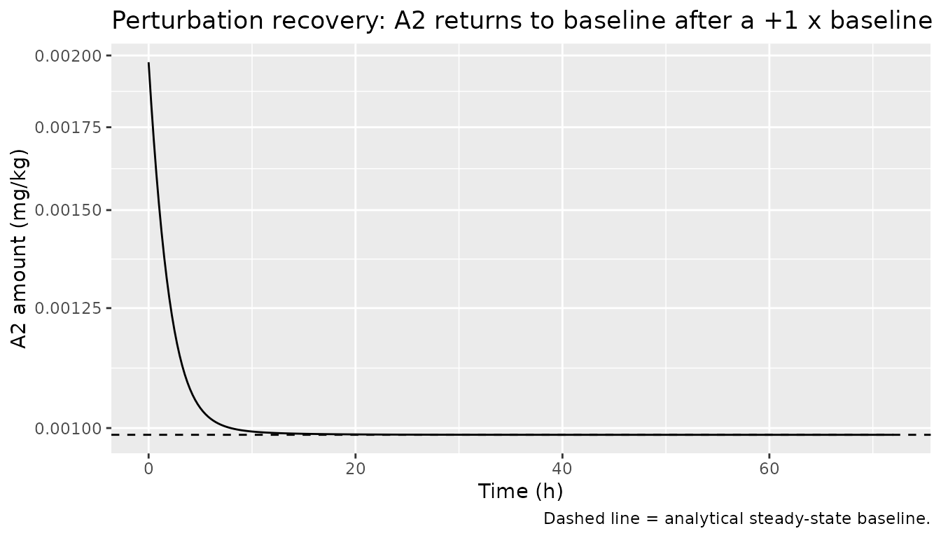
Half-life check
The paper reports half-lives of 3.33 h (A2), 2.83 d (A2B2), and 3.94
h (B) (Results section: “elimination rate constants translated easily to
half-lives…”). With each ke from ini(),
ln(2) / ke should reproduce those values.
halflives <- data.frame(
  species = c("A2", "A2B2", "B"),
  ke_per_hr = c(0.208, 0.0102, 0.176),
  t_half_paper = c("3.33 h", "2.83 d", "3.94 h"),
  t_half_computed_h = signif(log(2) / c(0.208, 0.0102, 0.176), 4)
)
knitr::kable(halflives, caption = "Half-life sanity check vs. Dodds 2005 Results.")| species | ke_per_hr | t_half_paper | t_half_computed_h |
|---|---|---|---|
| A2 | 0.2080 | 3.33 h | 3.332 |
| A2B2 | 0.0102 | 2.83 d | 67.960 |
| B | 0.1760 | 3.94 h | 3.938 |
Computed values: 3.33 h, 2.83 d, 3.94 h – all match the published values.
Mass-balance check at steady state
At steady state, every ODE’s right-hand side equals zero. We evaluate each flux at the typical-value baseline:
A2_ss   <- sim_ss$A2[1]
A2B2_ss <- sim_ss$A2B2[1]
B_ss    <- sim_ss$B[1]

InfA2 <- 0.000622; keA2 <- 0.208; Ka <- 6.59
InfB  <- 0.0121;   keB  <- 0.176; keA2B2 <- 0.0102

dA2_dt   <- InfA2 - keA2*A2_ss - Ka*A2_ss*B_ss
dB_dt    <- InfB  - keB*B_ss  - 2*Ka*A2_ss*B_ss
dA2B2_dt <-              -keA2B2*A2B2_ss + 3*Ka*A2_ss*B_ss

flux <- data.frame(
  ODE          = c("d/dt(A2)", "d/dt(B)", "d/dt(A2B2)"),
  rhs_mg_kg_hr = signif(c(dA2_dt, dB_dt, dA2B2_dt), 3)
)
knitr::kable(flux, caption = "Each RHS evaluated at the analytical SS; values are zero within rounding.")| ODE | rhs_mg_kg_hr |
|---|---|
| d/dt(A2) | 0 |
| d/dt(B) | 0 |
| d/dt(A2B2) | 0 |
Replicate Figure 6: single-dose and multiple-dose profiles
Dodds 2005 Figure 6 shows the typical-value predictions for a single 5 mg/kg IV bolus of rA2 (top panel) and 14 daily 6 mg/kg IV boluses (bottom panel), with 100 h of pre-dose baseline included on the time axis. The y-axis carries each of the three assay readings.
ev_single <- rxode2::et() |>
  rxode2::et(amt = 5, cmt = "A2", time = 0) |>
  rxode2::et(seq(-100, 30 * 24, by = 1), cmt = "total_a2_assay")
sim_single <- rxode2::rxSolve(mod_typical, ev_single) |> as.data.frame()
#> ℹ omega/sigma items treated as zero: 'etalke_dimer', 'etalke_tetramer', 'etalke_monomer'
#> Warning:
#> with negative times, compartments initialize at first negative observed time
#> with positive times, compartments initialize at time zero
#> use 'rxSetIni0(FALSE)' to initialize at first observed time
#> this warning is displayed once per session

sim_single_long <- sim_single |>
  dplyr::select(time, total_a2_assay, a2b2_assay, b_assay) |>
  tidyr::pivot_longer(-time, names_to = "assay", values_to = "conc_mg_L") |>
  dplyr::mutate(
    assay = factor(assay,
                   levels = c("total_a2_assay", "a2b2_assay", "b_assay"),
                   labels = c("Total A2 assay (A2 + A2B2)",
                              "A2B2 tetramer assay",
                              "Free B assay")))

ggplot(sim_single_long, aes(time, conc_mg_L, colour = assay, linetype = assay)) +
  geom_line() +
  geom_vline(xintercept = 0, alpha = 0.3) +
  labs(x = "Time relative to dose (h)",
       y = "Assay reading (mg/L)",
       colour = NULL, linetype = NULL,
       title = "Figure 6 (top): single 5 mg/kg IV bolus rA2",
       caption = "Solid line = A2B2 assay; broken line = total A2 assay; free B assay near 1.0 mg/L baseline (per Dodds 2005 Figure 6 caption).") +
  theme(legend.position = "bottom") +
  scale_y_continuous(limits = c(0, NA))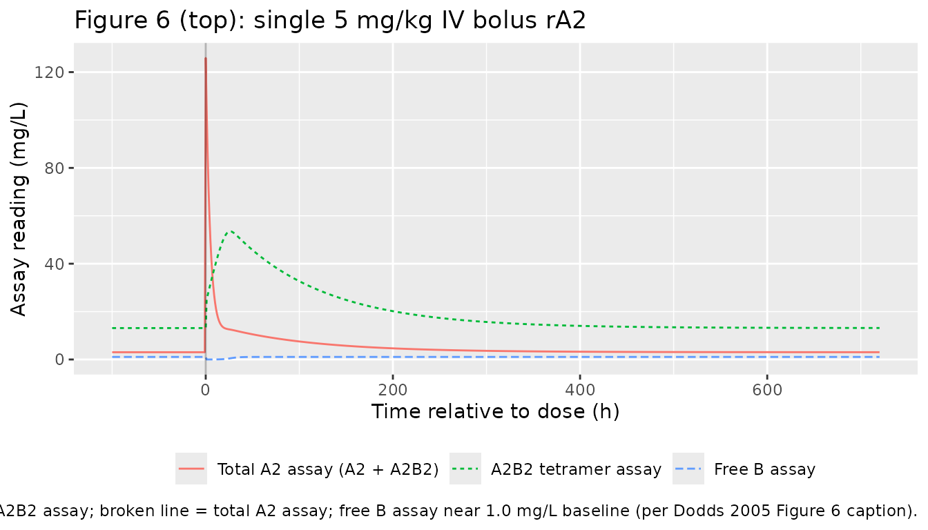
Replicates the top panel of Figure 6: typical-value response to a single 5 mg/kg IV bolus of rA2 at t = 0, with 100 h of pre-dose baseline.
ev_multi <- rxode2::et() |>
  rxode2::et(amt = 6, cmt = "A2", time = 0, ii = 24, addl = 13) |>
  rxode2::et(seq(-100, 30 * 24, by = 1), cmt = "total_a2_assay")
sim_multi <- rxode2::rxSolve(mod_typical, ev_multi) |> as.data.frame()
#> ℹ omega/sigma items treated as zero: 'etalke_dimer', 'etalke_tetramer', 'etalke_monomer'

sim_multi_long <- sim_multi |>
  dplyr::select(time, total_a2_assay, a2b2_assay, b_assay) |>
  tidyr::pivot_longer(-time, names_to = "assay", values_to = "conc_mg_L") |>
  dplyr::mutate(
    assay = factor(assay,
                   levels = c("total_a2_assay", "a2b2_assay", "b_assay"),
                   labels = c("Total A2 assay (A2 + A2B2)",
                              "A2B2 tetramer assay",
                              "Free B assay")))

ggplot(sim_multi_long, aes(time, conc_mg_L, colour = assay, linetype = assay)) +
  geom_line() +
  geom_vline(xintercept = 0, alpha = 0.3) +
  labs(x = "Time relative to first dose (h)",
       y = "Assay reading (mg/L)",
       colour = NULL, linetype = NULL,
       title = "Figure 6 (bottom): 6 mg/kg IV bolus rA2 daily for 14 days",
       caption = "Tetramer (A2B2) accumulates during the dosing window and decays with its 2.83-day half-life thereafter.") +
  theme(legend.position = "bottom") +
  scale_y_continuous(limits = c(0, NA))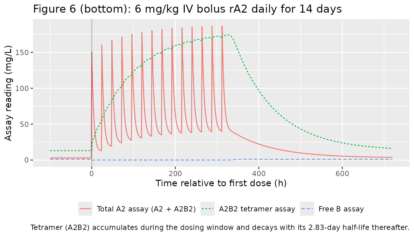
Replicates the bottom panel of Figure 6: typical-value response to 14 daily 6 mg/kg IV boluses of rA2, with 100 h of pre-dose baseline. Dose-induced accumulation of A2B2 builds over the dosing window and decays slowly thereafter.
Stochastic VPC (population variability)
The full population model carries IIV on the three elimination rate constants. A modest VPC at the 5 mg/kg single-dose level uses the published variances and residual errors directly.
set.seed(2005)
n_sub <- 100
times <- c(0, 0.25, 1, 2, 4, 8, 24, 72, 120, 168, 240, 336, 504, 672)
ev_vpc <- rxode2::et() |>
  rxode2::et(amt = 5, cmt = "A2", time = 0) |>
  rxode2::et(times, cmt = "total_a2_assay") |>
  rxode2::et(id = seq_len(n_sub))

sim_vpc <- rxode2::rxSolve(mod, ev_vpc) |> as.data.frame()
#> ℹ parameter labels from comments will be replaced by 'label()'

vpc_long <- sim_vpc |>
  dplyr::filter(time > 0) |>
  dplyr::select(id, time, total_a2_assay, a2b2_assay, b_assay) |>
  tidyr::pivot_longer(c(total_a2_assay, a2b2_assay, b_assay),
                      names_to = "assay", values_to = "conc_mg_L") |>
  dplyr::group_by(time, assay) |>
  dplyr::summarise(
    Q05 = quantile(conc_mg_L, 0.05, na.rm = TRUE),
    Q50 = quantile(conc_mg_L, 0.50, na.rm = TRUE),
    Q95 = quantile(conc_mg_L, 0.95, na.rm = TRUE),
    .groups = "drop"
  ) |>
  dplyr::mutate(
    assay = factor(assay,
                   levels = c("total_a2_assay", "a2b2_assay", "b_assay"),
                   labels = c("Total A2 assay (A2 + A2B2)",
                              "A2B2 tetramer assay",
                              "Free B assay")))

ggplot(vpc_long, aes(time, Q50)) +
  geom_ribbon(aes(ymin = Q05, ymax = Q95), alpha = 0.25) +
  geom_line() +
  facet_wrap(~ assay, scales = "free_y") +
  scale_y_log10() +
  labs(x = "Time (h)",
       y = "Assay reading (mg/L, log scale)",
       title = "Single 5 mg/kg IV rA2: typical median and 5-95% envelope",
       caption = paste0("Each panel: simulated median (line) and 5-95% percentiles ",
                        "(ribbon) across ", n_sub, " virtual cyno monkeys."))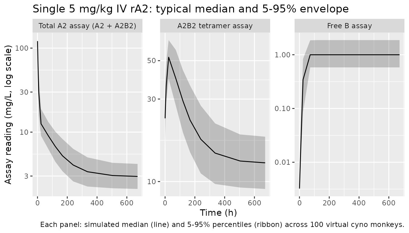
Stochastic 100-subject simulation at 5 mg/kg IV single dose: median and 5-95 percentile envelope for each assay output. Population variability sits on the three elimination rate constants only (paper Table 1).
Assumptions and deviations
-
No subject-level covariates. The published paper
does not report any covariate effects in the final model. Body weight is
baked into the mg/kg parameterisation throughout (Dodds 2005,
Population/Statistical Model: “Many of the parameters described so far
are, by construction, weight normalized.”). The
covariateDatalist is therefore empty. -
Paper-specific compartment and parameter names. The
state variables
A2,A2B2,Band the structural parameterske_*,inf_*,vt_dimer,v_tetramer,v_monomer,k_assocare paper-mechanistic and do not match the canonicalcentral/peripheral/ka/cl/vcfamily used by classical popPK models. Compartments are declared viapaper_specific_compartmentssocheckModelConventions()accepts them. The structural parameter names follow the lowercase snake-case convention recommended for endogenous / mechanistic models inreferences/parameter-names.md. -
Dose unit is mg/kg, not mg. Because every model
parameter is weight-normalised, the dosing event
amtmust be in mg/kg (the body mass of the animal cancels through the system and never appears explicitly). Theunits$dosingfield flags this; users must NOT multiply by body weight when constructing event tables. -
Single subjects share the same typical SS pre-dose
baseline. Per-subject baseline variability is implicit through
the IIV on the three elimination rate constants (which moves the
steady-state values via Equations 4-6 when an individual’s
ke_*differ from the typical values). -
IIV is log-normal. The paper reports
between-subject variances as NONMEM Omega values with units
%^2, with BSV computed assqrt(variance) x 100%. We encode them as variances on the log-scale eta (ke_i = exp(lke + eta_i)), which is the standard NONMEM exponential-IIV parameterisation. The reported BSV column (25.1%, 16.4%, 38.9%) equalssqrt(0.0629),sqrt(0.0268),sqrt(0.151). -
PKNCA omitted. Because the totalA2 ELISA cannot
separate recombinant rA2 from endogenous cA2 (they are functionally
identical and assay-indistinguishable), the dosed-drug signal cannot be
cleanly extracted from any of the three outputs without a
baseline-subtraction assumption the paper does not specify. The paper
itself reports no NCA parameters. We follow the endogenous-validation
pattern (steady-state hold, perturbation recovery, mass-balance,
dimensional analysis, Figure 6 replication) instead. See
references/endogenous-validation.md. - Between-study differences not modelled. The paper notes that A2B2 elimination appears faster in the multiple-dose study than in the single-dose study but did not introduce a study-level random effect (“the model had no provision for differences between the 2 studies”, Discussion). The packaged model reproduces this design decision.