Model and source
- Citation: Zhang F, Tagen M, Throm S, Mallari J, Miller L, Guy RK, Dyer MA, Williams RT, Roussel MF, Nemeth K, Zhu F, Zhang J, Lu M, Panetta JC, Boulos N, Stewart CF. Whole-body physiologically based pharmacokinetic model for nutlin-3a in mice after intravenous and oral administration. Drug Metab Dispos. 2011;39(1):15-21.
- Article: https://doi.org/10.1124/dmd.110.035915
Nutlin-3a is a small-molecule MDM2 inhibitor (MW 581.5 g/mol, PubChem CID 11433190) under preclinical investigation as a p53 reactivator in retinoblastoma, neuroblastoma, rhabdomyosarcoma, and acute lymphoblastic leukemia. Zhang et al. (2011) developed a whole-body PBPK model in adult C57BL/6 mice to characterize plasma + multi-tissue disposition after intravenous and oral dosing, and used the model to design preclinical dosing regimens targeting unbound concentrations above in-vitro IC50 values in retina, vitreous, adrenal gland, muscle, plasma, spleen, and bone marrow.
Population
The model was fit simultaneously to pooled plasma and tissue concentration-time data from two single-dose pharmacokinetic studies in adult C57BL/6 mice (Methods, p.16):
- Study 1: 145 mice (128 male + 17 female) split into three arms – oral 100 mg/kg, oral 200 mg/kg, and IV 10 mg/kg – with destructive sampling at nine timepoints (0.5, 1, 2, 4, 8, 12, 24, 36, 48 h) for plasma, liver, spleen, intestine, brain, vitreous, retina, and bone marrow.
- Study 2: 210 adult male mice in oral 50, oral 100, IV 10, and IV 20 mg/kg arms with serial plasma sampling and tissue sampling (lung, kidney, adrenal gland, muscle, fat, intestine) from the IV 20 mg/kg arm only.
Both studies used non-tumor-bearing adult animals, and the model is
therefore representative of typical (not tumor-altered) tissue
disposition. The same information is available programmatically via the
model’s population metadata
(readModelDb("Zhang_2011_nutlin3a")$population).
Source trace
The per-parameter origin is recorded as an in-file comment next to
each ini() entry in
inst/modeldb/specificDrugs/Zhang_2011_nutlin3a.R. The table
below collects them for review.
| Equation / parameter | Value | Source location |
|---|---|---|
| Eq for perfusion-limited tissue dA/dt | derivation | p.17 |
| Eq for liver compartment (hepatic artery + portal + linear elim.) | derivation | p.17 |
| Eq for intestine lumen (linear absorption ka) | derivation | p.17 |
| Eq for retina + vitreous coupled by PA_VIT | derivation | p.17 |
| Eq for residual diffusion-limited (vascular + tissue, PA_RES) | derivation | p.17 |
| Eq for lung (perfusion-limited, Q_BLO) | derivation | p.17 |
| Eq for arterial pool with saturable elimination | derivation | p.17 |
| Eq for Langmuir plasma protein binding (Cp,u from Cp) | derivation | p.16, Eq 3 |
| ka | 0.409 (1/h) | Table 2 |
| Ke | 0.0160 (L/h, see Assumptions) | Table 2 |
| Vmax | 0.0287 (mg/h, see Assumptions) | Table 2 |
| Km | 0.050 (mg/L, see Assumptions) | Table 2 |
| K_ADI | 1.61 | Table 2 |
| K_ADR | 2.05 | Table 2 |
| K_BRA | 0.055 | Table 2 |
| K_INT | 12.2 | Table 2 |
| K_LIV | 7.54 | Table 2 |
| K_LUN | 1.78 | Table 2 |
| K_MUS | 2.08 | Table 2 |
| K_RET | 4.01 | Table 2 |
| K_SPL | 2.72 | Table 2 |
| K_VIT | 0.012 | Table 2 |
| K_RES | 4.8 | Table 2 |
| PA_VIT | 0.0036 (L/h) | Table 2 |
| PA_RES | 0.0048 (L/h) | Table 2 |
| K_MRW (bone marrow) | 1.0 (fixed) | Not in Table 2 – see Assumptions |
| Tissue volumes (% body weight) | per tissue | Table 1 |
| Tissue blood flows Q_B (mL/h) | per tissue | Table 1 |
| V_VEN, V_ART split | 75 / 25 % of V_BLO | text p.17 |
| V_RES_VASC, V_RES_TIS split | 5 / 95 % of V_RES | text p.17 |
| Q_LIV = Q_HA + Q_SPL + Q_INT | sum | text p.17 |
| B/P ratio | 0.70 | Results p.18, Fig 2A |
| Bmax | 286 (uM) | Results p.18 |
| KA (binding) | 0.085 (1/uM) | Results p.18 |
| IIV ka | 31.2% CV | Table 2 |
| IIV Ke | 6.4% CV | Table 2 |
| IIV Vmax | 40.6% CV | Table 2 |
| Residual error | 35.6% (proportional) | Table 2 |
Units in the ODE system
The paper does not report units for the saturable-elimination parameters (V_max, K_m), the hepatic linear-elimination parameter K_e, or the permeability-surface products PA_VIT and PA_RES. The packaged model encodes them in mass-based units consistent with the mg/kg dosing regimen, the saturable-elimination magnitudes, and the paper’s prose that elimination is “very rapid at concentrations below 10 uM”:
| Quantity | Units |
|---|---|
| Time | h |
| Volumes | L (mouse tissue density assumed 1 kg/L) |
| Blood and inter-organ flows Q_i, PA_VIT, PA_RES | L/h |
| Amounts (state values) | mg |
| Concentrations (state / volume) | mg/L |
| ka | 1/h |
| Ke (hepatic linear elimination, applied to C_ART) | L/h |
| Vmax | mg/h |
| Km | mg/L |
| Partition coefficients K_i | unitless |
| Bmax, KA (binding) | uM and 1/uM, respectively (separate from ODE system) |
| Body weight (covariate column WT) | kg (mouse default 0.025 kg) |
Doses are supplied in mg. For a mg/kg dosing regimen, multiply by the animal’s body weight in kg.
Virtual cohort
The validation virtual cohort uses the five single-dose arms reported in the paper: IV 10 mg/kg, IV 20 mg/kg, oral 50 mg/kg, oral 100 mg/kg, and oral 200 mg/kg, each in 25 g (0.025 kg) typical C57BL/6 mice.
bw_kg <- 0.025          # typical adult C57BL/6 body weight
n_per_arm <- 1L          # typical-value (deterministic) simulation

make_cohort <- function(dose_mgkg, route, id_offset = 0L,
                        bw = bw_kg, n = n_per_arm) {
  dose_mg <- dose_mgkg * bw
  cmt_dose <- if (route == "iv") "venous" else "depot"
  arm <- sprintf("%s %d mg/kg", toupper(route), dose_mgkg)

  rxode2::et(amt = dose_mg, cmt = cmt_dose, time = 0) |>
    rxode2::et(time = seq(0, 48, by = 0.25)) |>
    as.data.frame() |>
    dplyr::mutate(id = 1L + id_offset,
                  treatment = arm,
                  dose_mgkg = dose_mgkg,
                  route = route,
                  WT = bw)
}

events <- dplyr::bind_rows(
  make_cohort(10,  "iv",   id_offset = 0L),
  make_cohort(20,  "iv",   id_offset = 1L),
  make_cohort(50,  "po",   id_offset = 2L),
  make_cohort(100, "po",   id_offset = 3L),
  make_cohort(200, "po",   id_offset = 4L)
)

stopifnot(!anyDuplicated(unique(events[, c("id", "time", "evid")])))
Simulation
mod <- readModelDb("Zhang_2011_nutlin3a")
mod_typical <- mod |> rxode2::zeroRe()
#> ℹ parameter labels from comments will be replaced by 'label()'
sim <- rxode2::rxSolve(
  mod_typical, events = events,
  keep = c("treatment", "dose_mgkg", "route", "WT")
) |> as.data.frame()
#> ℹ omega/sigma items treated as zero: 'etalka', 'etalkel', 'etalvmax'
#> Warning: multi-subject simulation without without 'omega'
Replicate published figure: tissue concentration-time
# Replicates Figure 3 of Zhang 2011: concentration-time plots of nutlin-3a
# in tissues (plasma and 9 perfused tissues) after a single IV 20 mg/kg
# bolus. The paper plots data from the IV 20 mg/kg group together with
# the model fit; here we render the typical-value prediction only.
plot_df <- sim |>
  dplyr::filter(treatment == "IV 20 mg/kg", time > 0, time <= 24) |>
  dplyr::transmute(
    time,
    Plasma   = Cc,
    Liver    = c_liv,
    Spleen   = c_spl,
    Intestine = c_int,
    Lung     = c_lun,
    Adipose  = c_adi,
    Muscle   = c_mus,
    Adrenal  = c_adr,
    Brain    = c_bra,
    Retina   = c_ret
  ) |>
  tidyr::pivot_longer(-time, names_to = "tissue", values_to = "conc")

ggplot(plot_df, aes(time, conc)) +
  geom_line() +
  facet_wrap(~tissue, ncol = 3, scales = "free_y") +
  scale_y_log10() +
  labs(x = "Time (h)", y = "Concentration (mg/L)",
       title = "Figure 3: Tissue concentration-time after IV 20 mg/kg",
       caption = "Replicates Figure 3 of Zhang 2011 (typical-value prediction).")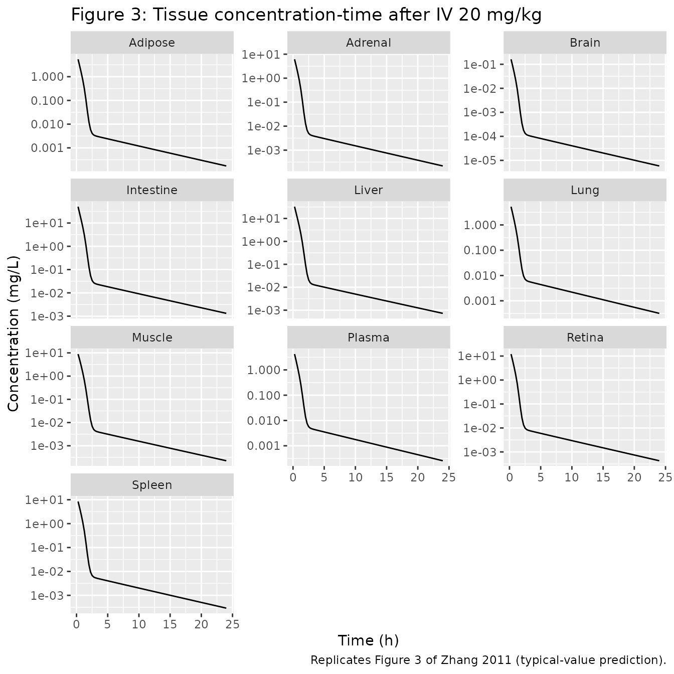
# Eye sub-system: retina and vitreous after oral 200 mg/kg.
eye_df <- sim |>
  dplyr::filter(treatment == "PO 200 mg/kg", time > 0, time <= 24) |>
  dplyr::transmute(time,
                   Retina = c_ret,
                   Vitreous = c_vit) |>
  tidyr::pivot_longer(-time, names_to = "tissue", values_to = "conc")

ggplot(eye_df, aes(time, conc, colour = tissue)) +
  geom_line() +
  scale_y_log10() +
  labs(x = "Time (h)", y = "Concentration (mg/L)",
       title = "Retina + vitreous after PO 200 mg/kg",
       caption = "Reproduces the ocular sub-system used by Zhang 2011 to design retinoblastoma dosing.")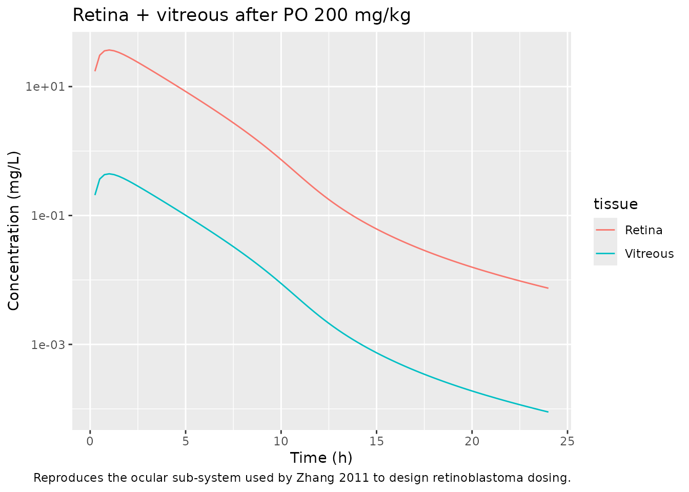
Replicate published figure: oral multiple-dose plasma profile
# Replicates Figure 4 of Zhang 2011: simulated plasma nutlin-3a after
# multiple oral 200 mg/kg doses given QD or BID.
make_md_cohort <- function(dose_mgkg, freq, id_offset = 0L,
                           bw = bw_kg, ndoses = 7L) {
  interval <- if (freq == "QD") 24 else 12
  dose_mg <- dose_mgkg * bw
  doses <- rxode2::et(time = seq(0, by = interval, length.out = ndoses),
                      amt = dose_mg, cmt = "depot")
  obs   <- rxode2::et(time = seq(0, ndoses * interval, by = 0.25))
  ev <- rxode2::etRbind(doses, obs)
  as.data.frame(ev) |>
    dplyr::mutate(id = 1L + id_offset,
                  treatment = sprintf("PO %d mg/kg %s", dose_mgkg, freq),
                  WT = bw)
}

md_events <- dplyr::bind_rows(
  make_md_cohort(200, "QD",  id_offset = 0L),
  make_md_cohort(200, "BID", id_offset = 1L)
)
stopifnot(!anyDuplicated(unique(md_events[, c("id", "time", "evid")])))

md_sim <- rxode2::rxSolve(mod_typical, events = md_events,
                          keep = c("treatment")) |>
  as.data.frame()
#> ℹ omega/sigma items treated as zero: 'etalka', 'etalkel', 'etalvmax'
#> Warning: multi-subject simulation without without 'omega'

ggplot(md_sim, aes(time, Cc, colour = treatment)) +
  geom_line() +
  scale_y_log10() +
  labs(x = "Time (h)", y = "Plasma nutlin-3a (mg/L)",
       title = "Figure 4: Plasma nutlin-3a after multiple oral 200 mg/kg doses",
       caption = "Replicates Figure 4 of Zhang 2011.")
#> Warning in scale_y_log10(): log-10 transformation introduced infinite values.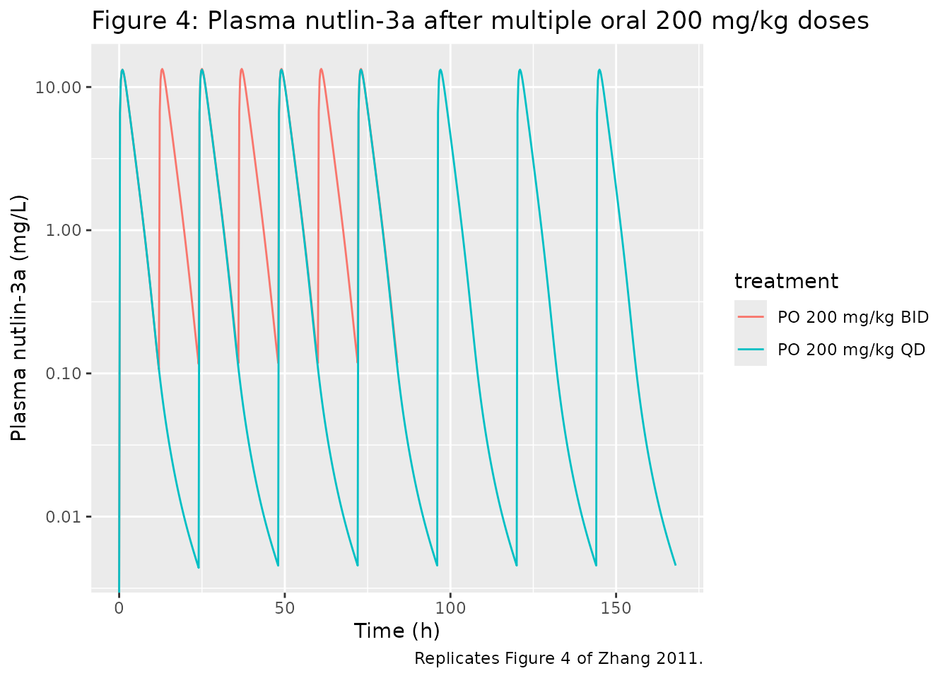
PKNCA validation
PKNCA is used to compute single-dose AUC and Cmax / Tmax for each of the five single-dose arms. The paper does not tabulate observed NCA parameters per dose-group (it reports model-derived AUC0-24 at steady state and bioavailability across dosing schedules), so the comparison below characterises the simulated single-dose exposures rather than a side-by-side observed-vs-simulated audit.
sim_nca <- sim |>
  dplyr::filter(time <= 48, !is.na(Cc)) |>
  dplyr::select(id, time, Cc, treatment)

conc_obj <- PKNCA::PKNCAconc(sim_nca, Cc ~ time | treatment + id)

dose_df <- events |>
  dplyr::filter(evid == 1) |>
  dplyr::transmute(id, time, amt, treatment)

dose_obj <- PKNCA::PKNCAdose(dose_df, amt ~ time | treatment + id)

intervals <- data.frame(
  start = 0, end = 24,
  cmax = TRUE, tmax = TRUE, aucinf.obs = TRUE,
  half.life = TRUE, auclast = TRUE
)

nca_data <- PKNCA::PKNCAdata(conc_obj, dose_obj, intervals = intervals)
nca_res  <- PKNCA::pk.nca(nca_data)
nca_summary <- summary(nca_res)
knitr::kable(nca_summary, caption = "Simulated single-dose plasma NCA per arm.")| start | end | treatment | N | auclast | cmax | tmax | half.life | aucinf.obs |
|---|---|---|---|---|---|---|---|---|
| 0 | 24 | IV 10 mg/kg | 1 | 19.2 | 389 | 0.000 | 5.03 | 19.2 |
| 0 | 24 | IV 20 mg/kg | 1 | 38.7 | 777 | 0.000 | 5.02 | 38.7 |
| 0 | 24 | PO 100 mg/kg | 1 | 22.0 | 6.51 | 1.00 | 4.06 | 22.0 |
| 0 | 24 | PO 200 mg/kg | 1 | 46.0 | 13.2 | 1.00 | 4.07 | 46.0 |
| 0 | 24 | PO 50 mg/kg | 1 | 10.2 | 3.16 | 1.00 | 3.99 | 10.2 |
Bioavailability check
Zhang et al. report predicted bioavailability of approximately 75% at 25 mg/kg QD rising to 91% at 400 mg/kg QD (text p.18). The single-dose 0-24 h AUC ratio (oral vs IV at matched dose) is a useful spot-check.
make_oral_iv_pair <- function(dose_mgkg, id_offset = 0L, bw = bw_kg) {
  dose_mg <- dose_mgkg * bw
  ev_iv <- rxode2::et(amt = dose_mg, cmt = "venous", time = 0) |>
    rxode2::et(time = seq(0, 24, by = 0.25)) |>
    as.data.frame() |>
    dplyr::mutate(id = 1L + id_offset,
                  treatment = sprintf("IV %d mg/kg", dose_mgkg),
                  WT = bw)
  ev_po <- rxode2::et(amt = dose_mg, cmt = "depot", time = 0) |>
    rxode2::et(time = seq(0, 24, by = 0.25)) |>
    as.data.frame() |>
    dplyr::mutate(id = 2L + id_offset,
                  treatment = sprintf("PO %d mg/kg", dose_mgkg),
                  WT = bw)
  dplyr::bind_rows(ev_iv, ev_po)
}

f_events <- dplyr::bind_rows(
  make_oral_iv_pair(100, id_offset = 100L),
  make_oral_iv_pair(200, id_offset = 200L)
)
f_sim <- rxode2::rxSolve(mod_typical, events = f_events,
                          keep = c("treatment")) |> as.data.frame()
#> ℹ omega/sigma items treated as zero: 'etalka', 'etalkel', 'etalvmax'
#> Warning: multi-subject simulation without without 'omega'

f_auc <- f_sim |>
  dplyr::filter(time > 0, time <= 24, !is.na(Cc)) |>
  dplyr::group_by(treatment) |>
  dplyr::arrange(time, .by_group = TRUE) |>
  dplyr::summarise(
    auc24 = sum(diff(time) * (head(Cc, -1) + tail(Cc, -1)) / 2),
    .groups = "drop"
  )
knitr::kable(f_auc, caption = "Simulated 0-24 h AUC by treatment.")| treatment | auc24 |
|---|---|
| IV 100 mg/kg | 9.601308 |
| IV 200 mg/kg | 19.657642 |
| PO 100 mg/kg | 21.608476 |
| PO 200 mg/kg | 45.183040 |
Assumptions and deviations
Units for V_max, K_m, K_e, PA_VIT, PA_RES are inferred. Table 2 reports point values without units. The packaged model assumes mg/h for V_max, mg/L for K_m, L/h for K_e (acting on C_ART, see next point), and L/h for the permeability-surface products. Under these units the saturable arm clears a ~0.5 mg bolus in ~17 h at high concentration (V_max ~ 0.0287 mg/h) and reaches an apparent clearance of V_max / K_m ~ 0.57 L/h at C << K_m, giving a half-life of ~1.5 min at low concentration that matches the paper’s narrative description of “very rapid” clearance below 10 uM (5.8 mg/L). Users who need a different unit system can override the corresponding
ini()values viarxSolve(params = c(lvmax = ..., lkm = ..., ...)).Hepatic linear elimination term acts on C_ART, not C_LIV. The paper’s liver ODE on p.17 literally writes
V_LIV * dA_LIV/dt = Q_LIV * (C_BLO,LIV - C_LIV/K_LIV) - k_e * C_ART, i.e. the linear elimination depends on the arterial concentration rather than the local liver concentration. The packaged model preserves this literal form. Mechanistically a more usual choice is- k_e * C_LIV(clearance from the local hepatic concentration); users who prefer that interpretation can swap the term inmodel()or refit K_e against the original data.Bone marrow partition coefficient K_MRW is not reported. Table 2 lists partition coefficients for ten tissues (adipose, adrenal, brain, intestine, liver, lung, muscle, retina, spleen, vitreous) plus the residual diffusion-limited compartment, but does not list a value for the bone-marrow perfusion-limited compartment. The model fixes
K_MRW = 1.0(fixed(log(1.0))) so the marrow compartment is parameter-complete and can be simulated; this is a documented gap, not an estimated value. A downstream user who has access to the underlying data can re-estimate it.Non-canonical tissue compartment names. The model uses physiology-named compartments (
venous,arterial,lung,liver,intestine,spleen,adipose,adrenal,brain,bonemarrow,muscle,retina,vitreous,res_vasc,res_tis) instead of the canonicalcentral/peripheral<n>/effectnames. This is the same accommodation already made forinst/modeldb/pharmacokinetics/Shah_2012_mAb_PBPK.Rand is unavoidable for PBPK models that need to identify each tissue by name.checkModelConventions()emits warnings for these names; they are intentional, not errors.Plasma protein binding is decoupled from the elimination ODEs. The Langmuir binding (B_max, K_A) is used to compute the unbound plasma concentration (
Cc_unbound) and unbound fraction (fub) reported alongsideCc, but the elimination ODEs operate on the total arterial / liver concentrations. This matches the paper’s formulation, where the unbound calculation is used downstream for tissue exposure / IC50 comparisons rather than fed back into the saturable / linear elimination.Body weight = 25 g default. The mouse studies report adult C57BL/6 mice; the packaged model defaults to
WT = 0.025kg, the typical adult body weight. Users can override via the event-table covariate columnWTorrxSolve(params = c(WT = ...)). All tissue volumes scale linearly withWT(assumed tissue density 1 kg/L). The blood flows are absolute (L/h) from Brown et al. 1997 for a standard mouse and are not scaled; for a substantially different body weight an allometric correction (Q_i ~ WT^0.75) would be appropriate.