Model and source
- Citation: Chen X, Wang DD, Xu H, Li ZP. Initial dose recommendation for sirolimus in paediatric kaposiform haemangioendothelioma patients based on population pharmacokinetics and pharmacogenomics. J Int Med Res. 2020;48(8):300060520947627. doi:10.1177/0300060520947627
- Description: One-compartment population PK model with first-order absorption for oral sirolimus in Chinese children with kaposiform haemangioendothelioma, developed from routine therapeutic-drug-monitoring trough concentrations (Chen 2020). Apparent clearance CL/F scales with body weight by a fixed allometric exponent of 0.75 and is 1.999-fold higher in CYP3A51 carriers (expressers) than in CYP3A53/*3 nonexpressers; apparent volume V/F scales linearly with body weight. Both are normalized to a 70 kg standard weight. The absorption rate constant is fixed at 0.485 per hour from the group’s earlier paediatric sirolimus model. Inter-individual variability is on CL/F only and the residual error is proportional.
- Article: https://doi.org/10.1177/0300060520947627
Chen and colleagues fit a one-compartment model with first-order absorption to routine trough concentrations of oral sirolimus from 14 Chinese children with kaposiform haemangioendothelioma, screening laboratory values, co-medications and an eight-gene pharmacogenomic panel. Body weight (with fixed allometric exponents) and CYP3A5 genotype were retained on apparent clearance. The paper’s practical output is a Monte Carlo initial-dose recommendation by CYP3A5 genotype and body weight (Figures 4 and 5) against a trough target of 10-15 ng/mL.
Population
A single-centre retrospective cohort treated at the Children’s Hospital of Fudan University, Shanghai, between March 2016 and July 2019 (Chen 2020 Table 1): 14 patients (9 male / 5 female), age 1.53 +/- 1.40 years and body weight 8.87 +/- 4.12 kg (mean +/- SD; ranges and medians were not reported). Oral sirolimus doses ranged 0.16-1.5 mg/day, adjusted by efficacy, adverse effects and therapeutic drug monitoring. Every concentration is a pre-dose trough, measured with the Emit 2000 Sirolimus Assay (linear range 3.5-30 ng/mL). One patient received phenobarbitone and two omeprazole.
CYP3A5 genotypes (Table 2) were *1/*1 in 1, *1/*3 in 6 and *3/*3 in 7 patients, so half the cohort are CYP3A5 expressers. ABCB1, ABCC4, ABCC8, CYP2C19, CYP3A4, UGT1A1 and UGT1A8 variants were also genotyped and screened, but not retained.
The same information is available programmatically via the model’s
population metadata
(readModelDb("Chen_2020_sirolimus")()$population).
Source trace
| Equation / parameter | Value | Source location |
|---|---|---|
lcl (CL/F at 70 kg, CYP3A5*3/*3) |
7.55 L/h | Table 3 (SE 15.2%); Equation vi |
lvc (V/F at 70 kg) |
1840 L | Table 3 (SE 12.7%); Equation vii |
lka (Ka) |
0.485 1/h, fixed | Table 3; Methods “Population pharmacokinetics model” |
e_wt_cl |
0.75, fixed | Methods “Covariate model”, Equation iii; Equation vi |
e_wt_vc |
1, fixed | Methods “Covariate model”, Equation iii; Equation vii |
e_cyp3a5_cl |
-0.999 | Table 3 (SE 40.3%); Equation vi |
etalcl |
0.121104 (omega = 0.348) | Table 3; Methods Equation i |
propSd |
0.390 | Table 3 (SE 7.3%); Methods Equation ii |
| Standard weight | 70 kg | Methods “Covariate model” (WTstd) |
CL/F = 7.55 * (WT/70)^0.75 * (1 - (-0.999) * CYP3A5) |
n/a | Equation vi (Results “Modelling and validation”) |
V/F = 1840 * (WT/70) |
n/a | Equation vii |
| CYP3A5 = 1 for a *1 carrier, 0 for *3/*3 | n/a | Results, text below Equation vii |
| Exponential IIV on CL/F only | n/a | Methods Equation i; Table 3 |
Proportional residual error C = (1 + eps1) * Y
|
n/a | Methods Equation ii; Table 3 footnote |
mod <- readModelDb("Chen_2020_sirolimus")
ui <- rxode2::rxode(mod)
#> ℹ parameter labels from comments will be replaced by 'label()'
theta <- ui$theta
CL_70 <- exp(theta[["lcl"]])
V_70 <- exp(theta[["lvc"]])
KA <- exp(theta[["lka"]])
CYP_FOLD <- 1 - theta[["e_cyp3a5_cl"]]
OMEGA_SD <- sqrt(ui$omega["etalcl", "etalcl"])
c(CL_70 = CL_70, V_70 = V_70, ka = KA, cyp3a5_fold = CYP_FOLD, omega_sd = OMEGA_SD)
#>       CL_70        V_70          ka cyp3a5_fold    omega_sd
#>       7.550    1840.000       0.485       1.999       0.348
Replicate Figure 3: typical CL/F per kg
Figure 3 of Chen 2020 plots the typical apparent clearance per kilogram against body weight for each genotype. It is pure arithmetic on Equation vi.
fig3 <- expand.grid(WT = c(5, 10, 20, 30, 40, 50, 60), CYP3A5_EXPR = 0:1) |>
  mutate(
    cl = CL_70 * (WT / 70)^theta[["e_wt_cl"]] * (1 - theta[["e_cyp3a5_cl"]] * CYP3A5_EXPR),
    cl_per_kg = cl / WT,
    genotype = ifelse(CYP3A5_EXPR == 1, "CYP3A5*1 carrier (B)", "CYP3A5*3/*3 (A)")
  )

ggplot(fig3, aes(WT, cl_per_kg, colour = genotype)) +
  geom_line() +
  geom_point() +
  labs(x = "Weight (kg)", y = "CL/F (L/h/kg)", colour = NULL,
       caption = "Replicates Figure 3 of Chen 2020.") +
  theme_bw()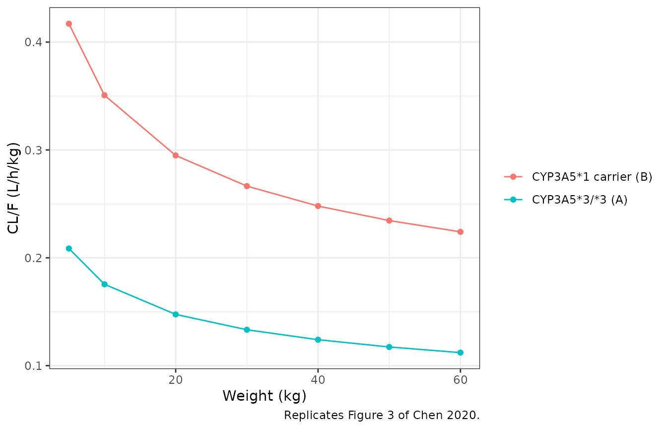
# Values read off Figure 3 (curve A, CYP3A5*3/*3) by the maintainers.
fig3_digitised <- c(0.208, 0.175, 0.147, 0.133, 0.123, 0.116, 0.111)
fig3_a <- fig3$cl_per_kg[fig3$CYP3A5_EXPR == 0]
fig3_b <- fig3$cl_per_kg[fig3$CYP3A5_EXPR == 1]
stopifnot(
  max(abs(fig3_a / fig3_digitised - 1)) < 0.02,
  # Results: "CL ... in CYP3A5*3/*3 and CYP3A5*1 were 1:1.999".
  all(abs(fig3_b / fig3_a - 1.999) < 1e-9)
)
Replicate Figures 4 and 5: the initial-dose simulations
Chen 2020 does not state the time point at which its initial-dose Monte Carlo evaluates the trough. The typical-value curves of Figure 4 identify it: the trough immediately before the fifth dose of a twice-daily regimen (48 h after the first dose) reproduces the printed curves to within the reading precision of the figure, while the troughs one dosing day earlier or later are roughly half and 1.4-fold as large. This is consistent with the paper’s framing of an initial dose. Note that the apparent half-life implied by the model is long (about 100 h for a CYP3A5*3/*3 child of the cohort’s mean weight), so this 48 h trough is far below steady state; see the steady-state section below.
Because the model is linear in dose and the trough is a monotone
function of etalcl, the percentiles and the probability of
target attainment in Figures 4 and 5 can be computed without sampling:
the 2.5th and 97.5th percentiles of the trough are the troughs at
etalcl = +/- 1.96 * omega, and the probability of a trough
in 10-15 ng/mL is the normal probability of the etalcl
interval that maps onto it. This removes Monte Carlo noise from the
comparison entirely.
# Trough 48 h after the first of four q12h doses, 1 mg per dose, on a fine eta
# grid; any mg/kg/day dose is then a linear rescale.
m0 <- rxode2::zeroRe(ui)
eta_grid <- seq(-5, 5, by = 0.01) * 0.6
ev1 <- rxode2::et(amt = 1, ii = 12, addl = 3, cmt = "depot") |>
  rxode2::et(48) |>
  as.data.frame()

trough_unit <- function(wt, cyp) {
  ev <- bind_rows(lapply(seq_along(eta_grid), function(i) {
    mutate(ev1, id = i, WT = wt, CYP3A5_EXPR = cyp)
  }))
  # zeroRe() removes the random effects, so rxode2 notes that a multi-subject
  # simulation has no omega; the etas are supplied explicitly in `params`.
  s <- suppressWarnings(rxode2::rxSolve(
    m0, ev, params = data.frame(etalcl = eta_grid), returnType = "data.frame"
  ))
  s <- s[s$time == 48, ]
  data.frame(WT = wt, CYP3A5_EXPR = cyp, eta = eta_grid[s$id], c_per_mg = s$Cc)
}
unit <- bind_rows(lapply(c(5, 10, 20, 30, 40, 50, 60), function(w) {
  bind_rows(trough_unit(w, 0), trough_unit(w, 1))
}))

# Trough at a given eta, by linear interpolation on the grid.
trough_at <- function(d, eta) approx(d$eta, d$c_per_mg, xout = eta)$y

band <- function(omega_sd, mgkgd) {
  unit |>
    group_by(WT, CYP3A5_EXPR) |>
    summarise(
      dose_mg = mgkgd * first(WT) / 2,
      median = dose_mg * trough_at(pick(everything()), 0),
      lo = dose_mg * trough_at(pick(everything()), 1.96 * omega_sd),
      hi = dose_mg * trough_at(pick(everything()), -1.96 * omega_sd),
      .groups = "drop"
    ) |>
    mutate(mgkgd = mgkgd)
}

# Probability that the 48 h trough is within 10-15 ng/mL. The trough falls as
# eta rises, so C >= 10 <=> eta <= eta(10) and C <= 15 <=> eta >= eta(15).
pta <- function(omega_sd, mgkgd) {
  unit |>
    group_by(WT, CYP3A5_EXPR) |>
    summarise(
      c = list(mgkgd * first(WT) / 2 * c_per_mg), eta = list(eta),
      .groups = "drop"
    ) |>
    rowwise() |>
    mutate(
      eta_hi = approx(rev(c), rev(eta), xout = 10, rule = 2)$y,
      eta_lo = approx(rev(c), rev(eta), xout = 15, rule = 2)$y,
      pta = 100 * max(0, pnorm(eta_hi / omega_sd) - pnorm(eta_lo / omega_sd))
    ) |>
    ungroup() |>
    transmute(WT, CYP3A5_EXPR, mgkgd = mgkgd, pta)
}
Figure 4: CYP3A5*3/*3
fig4 <- bind_rows(lapply(c(0.10, 0.20, 0.30), function(d) band(OMEGA_SD, d))) |>
  filter(CYP3A5_EXPR == 0)

ggplot(fig4, aes(WT, median, colour = factor(mgkgd))) +
  geom_line(linewidth = 1) +
  geom_line(aes(y = lo), linetype = "dashed") +
  geom_line(aes(y = hi), linetype = "dashed") +
  geom_hline(yintercept = c(10, 15), colour = "red", linetype = "dotted") +
  labs(x = "Weight (kg)", y = "Sirolimus trough at 48 h (ng/mL)",
       colour = "mg/kg/day\n(split q12h)",
       caption = "Replicates Figure 4 of Chen 2020 (median and 95% interval).") +
  theme_bw()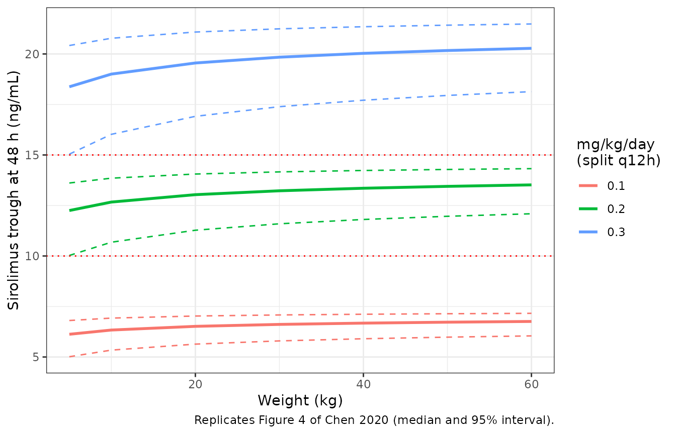
The table below compares the curves at the two ends of the weight axis with the values the maintainers read off Figure 4.
fig4_digitised <- tribble(
  ~mgkgd, ~WT, ~median, ~lo, ~hi,
  0.10, 5, 6.10, 4.95, 6.80,
  0.10, 60, 6.75, 6.00, 7.15,
  0.20, 5, 12.25, 9.95, 13.65,
  0.20, 60, 13.50, 12.05, 14.35,
  0.30, 5, 18.40, 14.90, 20.50,
  0.30, 60, 20.30, 18.05, 21.50
) |>
  pivot_longer(c(median, lo, hi), names_to = "quantity", values_to = "published")

fig4_cmp <- fig4 |>
  select(mgkgd, WT, median, lo, hi) |>
  pivot_longer(c(median, lo, hi), names_to = "quantity", values_to = "simulated") |>
  inner_join(fig4_digitised, by = c("mgkgd", "WT", "quantity")) |>
  mutate(pct_diff = 100 * (simulated / published - 1))

fig4_cmp |>
  rename(
    "Dose (mg/kg/day)" = mgkgd, "Weight (kg)" = WT, "Quantity" = quantity,
    "Model (ng/mL)" = simulated, "Figure 4 (ng/mL)" = published,
    "% difference" = pct_diff
  ) |>
knitr::kable(digits = 2)| Dose (mg/kg/day) | Weight (kg) | Quantity | Model (ng/mL) | Figure 4 (ng/mL) | % difference |
|---|---|---|---|---|---|
| 0.1 | 5 | median | 6.13 | 6.10 | 0.41 |
| 0.1 | 5 | lo | 5.01 | 4.95 | 1.28 |
| 0.1 | 5 | hi | 6.81 | 6.80 | 0.09 |
| 0.1 | 60 | median | 6.76 | 6.75 | 0.14 |
| 0.1 | 60 | lo | 6.04 | 6.00 | 0.75 |
| 0.1 | 60 | hi | 7.16 | 7.15 | 0.16 |
| 0.2 | 5 | median | 12.25 | 12.25 | 0.00 |
| 0.2 | 5 | lo | 10.03 | 9.95 | 0.77 |
| 0.2 | 5 | hi | 13.61 | 13.65 | -0.28 |
| 0.2 | 60 | median | 13.52 | 13.50 | 0.14 |
| 0.2 | 60 | lo | 12.09 | 12.05 | 0.33 |
| 0.2 | 60 | hi | 14.32 | 14.35 | -0.19 |
| 0.3 | 5 | median | 18.38 | 18.40 | -0.13 |
| 0.3 | 5 | lo | 15.04 | 14.90 | 0.94 |
| 0.3 | 5 | hi | 20.42 | 20.50 | -0.40 |
| 0.3 | 60 | median | 20.28 | 20.30 | -0.10 |
| 0.3 | 60 | lo | 18.13 | 18.05 | 0.47 |
| 0.3 | 60 | hi | 21.48 | 21.50 | -0.07 |
Figure 5: CYP3A5*1 carriers
fig5 <- bind_rows(lapply(c(0.10, 0.20, 0.23, 0.25, 0.30), function(d) {
  pta(OMEGA_SD, d)
})) |>
  filter(CYP3A5_EXPR == 1)

ggplot(fig5, aes(WT, pta, colour = factor(mgkgd))) +
  geom_line() +
  geom_point() +
  labs(x = "Weight (kg)", y = "Probability of a 10-15 ng/mL trough (%)",
       colour = "mg/kg/day\n(split q12h)",
       caption = "Replicates Figure 5 of Chen 2020.") +
  theme_bw()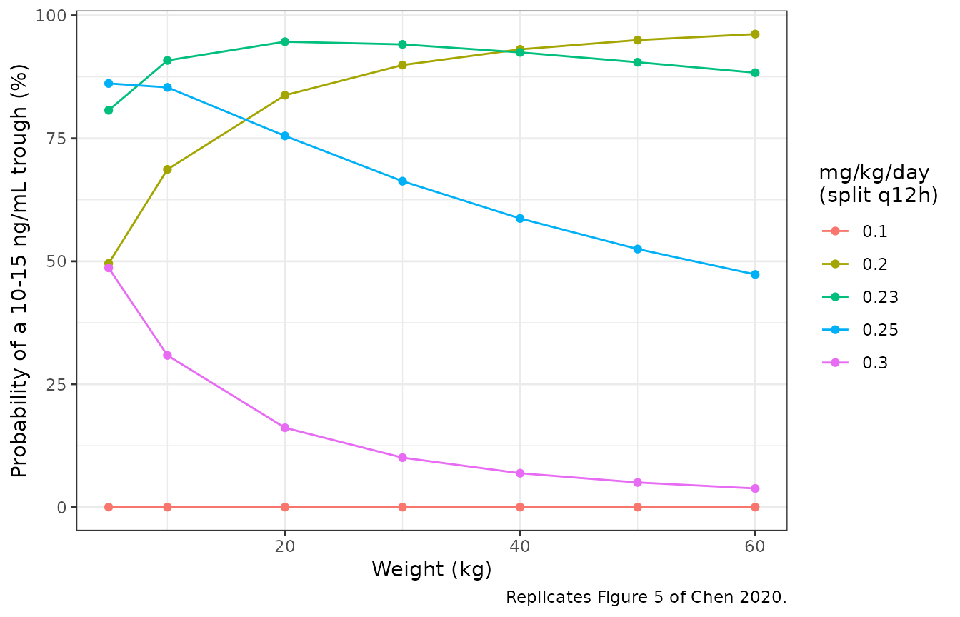
# Values read off Figure 5 by the maintainers.
fig5_digitised <- tribble(
  ~mgkgd, ~`5`, ~`10`, ~`20`, ~`30`, ~`40`, ~`50`, ~`60`,
  0.10, 0, 0, 0, 0, 0, 0, 0,
  0.20, 51, 71, 85, 90, 93, 94.5, 95.5,
  0.23, 83, 91, 93, 92, 91, 88, 86,
  0.25, 84.5, 82, 73, 64, 56, 51, 46,
  0.30, 47, 29, 15, 10, 7, 5.5, 4.5
) |>
  pivot_longer(-mgkgd, names_to = "WT", values_to = "published") |>
  mutate(WT = as.numeric(WT))

fig5_cmp <- inner_join(fig5, fig5_digitised, by = c("mgkgd", "WT")) |>
  mutate(diff = pta - published)

fig5_cmp |>
  select(mgkgd, WT, pta, published, diff) |>
  rename(
    "Dose (mg/kg/day)" = mgkgd, "Weight (kg)" = WT, "Model PTA (%)" = pta,
    "Figure 5 PTA (%)" = published, "Difference (points)" = diff
  ) |>
knitr::kable(digits = c(2, 0, 1, 1, 1))| Dose (mg/kg/day) | Weight (kg) | Model PTA (%) | Figure 5 PTA (%) | Difference (points) |
|---|---|---|---|---|
| 0.10 | 5 | 0.0 | 0.0 | 0.0 |
| 0.10 | 10 | 0.0 | 0.0 | 0.0 |
| 0.10 | 20 | 0.0 | 0.0 | 0.0 |
| 0.10 | 30 | 0.0 | 0.0 | 0.0 |
| 0.10 | 40 | 0.0 | 0.0 | 0.0 |
| 0.10 | 50 | 0.0 | 0.0 | 0.0 |
| 0.10 | 60 | 0.0 | 0.0 | 0.0 |
| 0.20 | 5 | 49.6 | 51.0 | -1.4 |
| 0.20 | 10 | 68.7 | 71.0 | -2.3 |
| 0.20 | 20 | 83.8 | 85.0 | -1.2 |
| 0.20 | 30 | 89.9 | 90.0 | -0.1 |
| 0.20 | 40 | 93.1 | 93.0 | 0.1 |
| 0.20 | 50 | 95.0 | 94.5 | 0.5 |
| 0.20 | 60 | 96.2 | 95.5 | 0.7 |
| 0.23 | 5 | 80.7 | 83.0 | -2.3 |
| 0.23 | 10 | 90.8 | 91.0 | -0.2 |
| 0.23 | 20 | 94.6 | 93.0 | 1.6 |
| 0.23 | 30 | 94.1 | 92.0 | 2.1 |
| 0.23 | 40 | 92.5 | 91.0 | 1.5 |
| 0.23 | 50 | 90.5 | 88.0 | 2.5 |
| 0.23 | 60 | 88.4 | 86.0 | 2.4 |
| 0.25 | 5 | 86.2 | 84.5 | 1.7 |
| 0.25 | 10 | 85.4 | 82.0 | 3.4 |
| 0.25 | 20 | 75.5 | 73.0 | 2.5 |
| 0.25 | 30 | 66.3 | 64.0 | 2.3 |
| 0.25 | 40 | 58.7 | 56.0 | 2.7 |
| 0.25 | 50 | 52.5 | 51.0 | 1.5 |
| 0.25 | 60 | 47.3 | 46.0 | 1.3 |
| 0.30 | 5 | 48.7 | 47.0 | 1.7 |
| 0.30 | 10 | 30.8 | 29.0 | 1.8 |
| 0.30 | 20 | 16.1 | 15.0 | 1.1 |
| 0.30 | 30 | 10.1 | 10.0 | 0.1 |
| 0.30 | 40 | 6.9 | 7.0 | -0.1 |
| 0.30 | 50 | 5.0 | 5.5 | -0.5 |
| 0.30 | 60 | 3.8 | 4.5 | -0.7 |
What Figures 4 and 5 say about the scale of omega
Table 3 prints omega CL/F = 0.348 without saying whether
this is the NONMEM variance or its square root. The Methods define the
variance as omega squared, which suggests an SD, and the paper’s own
simulations settle it: the 95% bands of Figure 4 and the
target-attainment curve of Figure 5 are reproduced above with an SD of
0.348, whereas reading 0.348 as a variance (SD 0.590) widens the Figure
4 bands well past what is printed.
alt <- band(sqrt(0.348), 0.20) |> filter(CYP3A5_EXPR == 0, WT %in% c(5, 60))
chosen <- band(OMEGA_SD, 0.20) |> filter(CYP3A5_EXPR == 0, WT %in% c(5, 60))
published_lo <- c(9.95, 12.05)
tibble(
  `Weight (kg)` = c(5, 60),
  `Figure 4 lower bound` = published_lo,
  `omega as SD (0.348)` = chosen$lo,
  `omega as variance (SD 0.590)` = alt$lo
) |>
knitr::kable(digits = 2)| Weight (kg) | Figure 4 lower bound | omega as SD (0.348) | omega as variance (SD 0.590) |
|---|---|---|---|
| 5 | 9.95 | 10.03 | 7.96 |
| 60 | 12.05 | 12.09 | 10.59 |
Virtual cohort
A cohort matching Table 1: body weight normal with mean 8.87 kg and SD 4.12 kg, redrawn (not clamped) outside 3-20 kg, and CYP3A5 expressers at the observed 50%. Each child receives the paper’s recommended initial dose for their genotype and weight: 0.20 mg/kg/day for CYP3A5*3/*3 and 0.23 mg/kg/day for CYP3A5*1 carriers below 30 kg, split every 12 h.
set.seed(2020)
rxode2::rxSetSeed(2020)
N_SUBJ <- 200
draw_wt <- function(n) {
  out <- numeric(0)
  while (length(out) < n) {
    x <- rnorm(n, 8.87, 4.12)
    out <- c(out, x[x >= 3 & x <= 20])
  }
  out[seq_len(n)]
}
cohort <- tibble(
  id = seq_len(N_SUBJ),
  WT = draw_wt(N_SUBJ),
  CYP3A5_EXPR = rbinom(N_SUBJ, 1, 0.5)
) |>
  mutate(mgkgd = ifelse(CYP3A5_EXPR == 1, 0.23, 0.20), dose = mgkgd * WT / 2)
Simulation: the first four weeks
TAU <- 12
N_DOSE <- 400 # 200 days: long enough for steady state in the slowest subject
SS_START <- (N_DOSE - 1) * TAU
obs_times <- sort(unique(c(seq(0, 24 * 28, by = 12), SS_START + seq(0, TAU, by = 0.25))))

events <- bind_rows(lapply(seq_len(N_SUBJ), function(i) {
  rxode2::et(amt = cohort$dose[i], ii = TAU, addl = N_DOSE - 1, cmt = "depot") |>
    rxode2::et(obs_times, cmt = "central") |>
    as.data.frame() |>
    mutate(id = i, WT = cohort$WT[i], CYP3A5_EXPR = cohort$CYP3A5_EXPR[i])
}))

sim <- rxode2::rxSolve(mod, events, keep = c("WT", "CYP3A5_EXPR"),
                       returnType = "data.frame") |>
  mutate(genotype = ifelse(CYP3A5_EXPR == 1, "CYP3A5*1 carrier", "CYP3A5*3/*3"))
#> ℹ parameter labels from comments will be replaced by 'label()'
stopifnot(dplyr::n_distinct(sim$id) == N_SUBJ)

sim |>
  filter(time <= 24 * 28, time %% 12 == 0) |>
  group_by(genotype, time) |>
  summarise(
    q05 = quantile(Cc, 0.05), q50 = median(Cc), q95 = quantile(Cc, 0.95),
    .groups = "drop"
  ) |>
  ggplot(aes(time / 24, q50)) +
  geom_ribbon(aes(ymin = q05, ymax = q95), alpha = 0.3) +
  geom_line() +
  geom_hline(yintercept = c(10, 15), colour = "red", linetype = "dotted") +
  facet_wrap(~genotype) +
  labs(x = "Day of therapy", y = "Sirolimus trough (ng/mL)",
       caption = "Median and 90% interval (no residual error) at the recommended initial dose.") +
  theme_bw()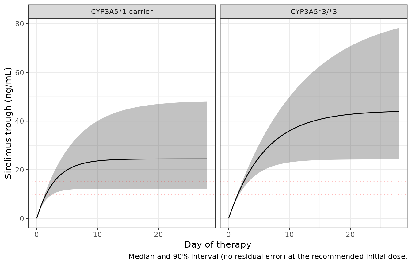
The troughs keep rising well after the 48 h point at which the paper evaluated the dose, because the model’s apparent half-life is about 100 h for a CYP3A5*3/*3 child of the cohort’s mean weight (about 50 h in a CYP3A5*1 carrier). At the recommended initial doses the median trough crosses the upper end of the 10-15 ng/mL target within the first week.
PKNCA validation
The paper reports no non-compartmental analysis, so there is no
published Cmax / AUC table to compare. PKNCA is instead run over the
final dosing interval at steady state and checked against the identity
AUC0-tau = Dose / CL, which holds per subject for a linear
model.
conc <- sim |>
  filter(!is.na(Cc), time >= SS_START) |>
  mutate(treatment = sprintf("%.2f mg/kg/day", ifelse(CYP3A5_EXPR == 1, 0.23, 0.20))) |>
  select(id, time, Cc, treatment)
dose <- events |>
  filter(evid == 1) |>
  select(id, amt) |>
  distinct() |>
  mutate(time = SS_START) |>
  left_join(distinct(conc, id, treatment), by = "id")

res <- PKNCA::pk.nca(PKNCA::PKNCAdata(
  PKNCA::PKNCAconc(conc, Cc ~ time | treatment + id, concu = "ng/mL", timeu = "h"),
  PKNCA::PKNCAdose(dose, amt ~ time | treatment + id, doseu = "mg"),
  intervals = data.frame(start = SS_START, end = SS_START + TAU,
                         cmax = TRUE, cmin = TRUE, cav = TRUE, auclast = TRUE)
))
nca <- as.data.frame(res$result)

nca |>
  group_by(treatment, PPTESTCD) |>
  summarise(median = median(PPORRES), .groups = "drop") |>
  pivot_wider(names_from = PPTESTCD, values_from = median) |>
  rename(
    "Treatment" = treatment,
    "AUC0-tau,ss (ng*h/mL)" = auclast,
    "Cmax,ss (ng/mL)" = cmax,
    "Cmin,ss (ng/mL)" = cmin,
    "Cavg,ss (ng/mL)" = cav
  ) |>
knitr::kable(digits = 1, caption = "Median steady-state exposure at the recommended initial doses.")| Treatment | AUC0-tau,ss (ng*h/mL) | Cavg,ss (ng/mL) | Cmax,ss (ng/mL) | Cmin,ss (ng/mL) |
|---|---|---|---|---|
| 0.20 mg/kg/day | 547.2 | 45.6 | 46.4 | 44.4 |
| 0.23 mg/kg/day | 310.6 | 25.9 | 26.8 | 24.5 |
auc_chk <- nca |>
  filter(PPTESTCD == "auclast") |>
  select(id, auc = PPORRES) |>
  left_join(sim |> distinct(id, cl), by = "id") |>
  left_join(cohort |> select(id, dose), by = "id") |>
  mutate(pct_diff = 100 * (auc * cl / 1000 / dose - 1))

stopifnot(
  nrow(auc_chk) == N_SUBJ,
  # 200 days is > 12 half-lives for the slowest simulated subject and the
  # trapezoid on a 15-minute grid is near exact, so this is tight.
  abs(median(auc_chk$pct_diff)) < 0.5,
  quantile(abs(auc_chk$pct_diff), 0.9) < 1
)
Assumptions and deviations
- Simulation time point of Figures 4 and 5. Not stated in the paper. The trough 48 h after the first of four twice-daily doses reproduces the Figure 4 typical-value curves to within the precision of reading the figure; that time point is used for the replication. The model parameters were not adjusted.
-
Scale of omega. Table 3 prints
omega CL/F = 0.348. It is taken as an SD (variance 0.348^2 = 0.121104) because the Methods define the variance as omega squared and because only this reading reproduces the 95% bands of Figure 4 and the probabilities of Figure 5 (section above). -
Scale of the residual error.
sigma 1 = 0.390is printed in the same notation as the omega row and is taken likewise as an SD (39% proportional). No figure in the paper independently discriminates this, and the residual error does not enter the paper’s dose simulations. -
CYP3A5 coefficient sign. Equation vi prints
(1 - (-0.999) * CYP3A5)and Table 3 prints -0.999; the model keeps the printed coefficient and form, which gives the 1:1.999 clearance ratio the Results state. - Whole-blood matrix. The paper names the Emit 2000 assay but not the matrix; the assay is a whole-blood method, as for the other sirolimus models in this library.
- Steady state versus the initial-dose target. With V/F = 1840 L at 70 kg the model’s apparent half-life is about 100 h in a 9 kg CYP3A5*3/*3 child, so troughs at the recommended initial doses rise several-fold beyond the 48 h value before reaching steady state. The paper’s recommendations concern the first days of therapy; subsequent dose adjustment by therapeutic drug monitoring is assumed.
- Figure 2 (prediction-corrected VPC) is not reproduced: the individual dosing histories over up to about 40,000 h of therapy are not available.
- Virtual cohort. Weight ranges were not reported; weights were drawn from a normal distribution with the Table 1 mean and SD, restricted to 3-20 kg.