Alisertib global popPK and exposure-safety (Zhou 2018)
Source:vignettes/articles/Zhou_2018_alisertib.Rmd
Zhou_2018_alisertib.RmdModel and source
- Citation: Zhou X, Mould DR, Takubo T, Sheldon-Waniga E, Huebner D, Milton A, Venkatakrishnan K. Global population pharmacokinetics of the investigational Aurora A kinase inhibitor alisertib in cancer patients: rationale for lower dosage in Asia. Br J Clin Pharmacol. 2018;84(1):35-51. doi:10.1111/bcp.13430. Structural and covariate equations from Figure 1; final parameter estimates from Table 5; the updated final model refitted on the combined analysis plus validation data is Supplementary Table S1 and is NOT the model packaged here.
- Article: https://doi.org/10.1111/bcp.13430
- Supplement (Table S1, the updated final model): http://onlinelibrary.wiley.com/doi/10.1111/bcp.13430/suppinfo
This paper contributes four models to
nlmixr2lib:
models <- c(
  "Zhou_2018_alisertib",
  "Zhou_2018_alisertib_neutropenia",
  "Zhou_2018_alisertib_stomatitis",
  "Zhou_2018_alisertib_diarrhea"
)
ui <- lapply(models, \(n) rxode2::rxode(readModelDb(n)))
#> ℹ parameter labels from comments will be replaced by 'label()'
names(ui) <- models

tibble::tibble(
  Model = models,
  Kind = c(
    "Population PK (2-compartment, 4-transit absorption)",
    "Exposure-safety logistic: grade >= 3 neutropenia",
    "Exposure-safety logistic: grade >= 2 stomatitis",
    "Exposure-safety logistic: grade >= 2 diarrhoea"
  ),
  n = c(422L, 591L, 593L, 594L)
) |>
knitr::kable(caption = "Models extracted from Zhou 2018.")| Model | Kind | n |
|---|---|---|
| Zhou_2018_alisertib | Population PK (2-compartment, 4-transit absorption) | 422 |
| Zhou_2018_alisertib_neutropenia | Exposure-safety logistic: grade >= 3 neutropenia | 591 |
| Zhou_2018_alisertib_stomatitis | Exposure-safety logistic: grade >= 2 stomatitis | 593 |
| Zhou_2018_alisertib_diarrhea | Exposure-safety logistic: grade >= 2 diarrhoea | 594 |
Alisertib (MLN8237) is an investigational selective Aurora A kinase inhibitor. The analysis pooled 10 clinical studies to ask a specific regulatory question: why is the maximum tolerated dose 50 mg twice daily in the West but only 30 mg twice daily in East Asia? The answer the model gives is a 52% higher relative bioavailability in patients enrolled in East Asia, and the paper uses that to justify a 40% lower regional dose.
Population
The model packaged here was fitted to the 422-patient analysis data set: adults with advanced haematological (43%) and nonhaematological (57%) malignancies, median age 62 years (range 21-85), median weight 73.3 kg (42.6-175.0), median BSA 1.84 m^2 (1.36-2.97), 46% female. 363 were enrolled in Western countries and 59 in the East Asian region (Japan; and Singapore, Taiwan, Hong Kong, South Korea). Alisertib was given orally at 5-150 mg once or twice daily under nil-per-os conditions. A further 249 patients – the phase II portion of study C14007, entirely Western – formed an external validation set. Baseline demographics are Zhou 2018 Tables 2 (continuous) and 3 (categorical); the study list is Table 1.
str(ui[["Zhou_2018_alisertib"]]$population, max.level = 1)
#> List of 16
#>  $ species       : chr "human"
#>  $ n_subjects    : int 422
#>  $ n_studies     : int 10
#>  $ age_range     : chr "21 to 85 years (analysis set); 21 to 88 years across the combined 671-patient data set"
#>  $ age_median    : chr "62 years"
#>  $ weight_range  : chr "42.6 to 175.0 kg (analysis set)"
#>  $ weight_median : chr "73.3 kg"
#>  $ bsa_range     : chr "1.36 to 2.97 m^2 (analysis set)"
#>  $ bsa_median    : chr "1.84 m^2"
#>  $ sex_female_pct: num 46
#>  $ race_ethnicity: Named num [1:5] 77 14 5 1 2
#>   ..- attr(*, "names")= chr [1:5] "White" "Asian (all)" "Black" "Other" ...
#>  $ disease_state : chr "Advanced haematological (43 percent) and nonhaematological (57 percent) malignancies"
#>  $ dose_range    : chr "5 to 150 mg alisertib orally once or twice daily, under nil-per-os conditions (no food from 2 h before until 1 "| __truncated__
#>  $ regions       : chr "Western countries (7 studies, 363 of 422 analysis-set patients); Japan (2 studies) and Singapore / Taiwan / Hon"| __truncated__
#>  $ renal_function: chr "Creatinine clearance 27.1 to 241.0 mL/min (analysis set); no effect on CL/F was detected over this range"
#>  $ notes         : chr "Baseline demographics are Table 2 (continuous) and Table 3 (categorical) of Zhou 2018; the study list is Table "| __truncated__
Molar units, and the mg-to-nmol conversion
Every concentration in Zhou 2018 is molar: the
additive residual error is reported in nmol/L, Figure 4 plots nmol/L,
and the exposure tables are in nM.h and uM.h. The packaged model
therefore works in nmol and nmol/L, and a dose in milligrams must be
converted before it is given to rxSolve().
The molar mass is not stated anywhere in the paper, so it is taken from an external source and flagged as such throughout (see Assumptions and deviations). The paper’s own simulation output corroborates it closely.
# NOT FROM THE PAPER: alisertib is C27H20ClFN4O4, molar mass 518.92 g/mol
# (PubChem CID 24771867 / the published structure). Zhou 2018 reports no
# molar mass, but its own simulated exposures reproduce under this value --
# checked explicitly in the "Figure 6" section below.
MW_ALISERTIB <- 518.92
mg_to_nmol <- function(mg) mg / MW_ALISERTIB * 1e6

dose_west <- mg_to_nmol(50)
dose_east <- mg_to_nmol(30)
c(`50 mg (nmol)` = dose_west, `30 mg (nmol)` = dose_east)
#> 50 mg (nmol) 30 mg (nmol)
#>     96353.97     57812.38
Source trace
Each ini() entry in the four model files carries its own
in-file provenance comment. They are collected here for review.
| Model | Equation / parameter | Value | Source location |
|---|---|---|---|
| PK |
lcl (CL/F) |
4.11 L/h | Table 5, row CL/F (SE 3.1%) |
| PK |
lvc (V1/F) |
54.3 L | Table 5, row V1/F (SE 3.9%) |
| PK |
lq (Q/F) |
7.07 L/h | Table 5, row Q/F (SE 10.9%) |
| PK |
lvp (V2/F) |
28.7 L | Table 5, row V2/F (SE 10%) |
| PK |
lktr (KTR) |
4.17 1/h | Table 5, row KTR (SE 3%) |
| PK |
e_region_eastasia_f (RGNF) |
-0.341 | Table 5, row RGNF (SE 11%); sign from the Table 5 footnote and Supplementary Table S1 |
| PK |
e_bsa_vc (BSAV1) |
0.899 | Table 5, row BSAV1 (SE 26.3%) |
| PK | BSA reference | 1.84 m^2 | Figure 1 equation (BSA/1.84)^BSAV1; the
Table 2 median |
| PK | IIV block (log SD) | 0.518 / 0.412 / 1.044 / 0.54 | Table 5, ‘IIV, ratio’ column for CL/F, V1/F, V2/F, KTR |
| PK | IIV correlations | 0.582, 0.509, 0.085, 0.116, 0.255, 0.025 | Table 5, lower-triangular correlation block |
| PK |
propSd (CCV) |
0.491 | Table 5, row CCV (SE 3.5%) |
| PK |
addSd (ADD) |
0 (fixed) | Table 5, row ADD; footnote b ‘automatically set to zero by the SAEM estimation algorithm’ |
| PK | 4-transit absorption chain; dose into transit1 | n/a | Figure 1 schematic; confirmed by Results ‘net mean transit time 0.96 h’ = 4/KTR |
| PK | Regional multiplier (1 + f) on CL/F, V1/F,
Q/F, V2/F |
n/a | Figure 1 equations |
| PK | No IIV on Q/F | n/a | Figure 1 (Q/F written without an exponential term); Table 5 IIV cell blank; Methods ‘the effect of removing BSV from Q/F was examined’ |
| ER | logistic form
logit(p) = b0 + b1*log(AUC)
|
n/a | Methods, ‘Exposure-safety analyses’; confirmed by the shape of the Figure 7 curves |
| ER neutropenia |
logit_ref / e_auc_logit
|
-2.316 / 0.675 | DIGITISED from Figure 7 panel A – not tabulated in the source |
| ER stomatitis |
logit_ref / e_auc_logit
|
-6.485 / 1.434 | DIGITISED from Figure 7 panel B – not tabulated in the source |
| ER diarrhoea |
logit_ref / e_auc_logit
|
-3.752 / 0.677 | DIGITISED from Figure 7 panel C – not tabulated in the source |
Which Table is the final model?
Zhou 2018 reports the model twice. Table 5 is the final model fitted to the 422-patient analysis set; Supplementary Table S1 is an updated final model refitted after the 249-patient validation set was folded in. Every row differs. Table 5 is what is packaged here; S1 is recorded below so a reader is not misled by a value that looks like a transcription error.
| Parameter | Table 5 (packaged) | Table S1 (updated) |
|---|---|---|
| CL/F (L/h) | 4.11 | 3.91 |
| V1/F (L) | 54.3 | 51.8 |
| Q/F (L/h) | 7.07 | 7.53 |
| V2/F (L) | 28.7 | 27.4 |
| KTR (1/h) | 4.17 | 3.93 |
| RGNF | 0.341 (sign dropped) | -0.325 |
| BSAV1 | 0.899 | 0.79 |
| CCV | 0.491 | 0.477 |
| ADD (nmol/L) | 0 (fixed) | 4.8 |
Note the RGNF row: the main-text Table 5 prints the magnitude
0.341 with a footnote reading “the affected parameters were
multiplied by (1-0.341)”, while the supplement prints
-0.325 with its minus sign under the
identical footnote wording. Figure 1 writes the effect as a multiplier
(1 + f). Taken together these settle the sign that
main-text typesetting dropped: the packaged coefficient is
-0.341, the multiplier is 0.659, and
1/0.659 = 1.517 recovers the “51.7% higher F” quoted in
Results.
Closed-form structural gates
Three quantities are fully determined by the Table 5 point estimates and are quoted independently in the paper’s Results text. They are exact arithmetic – no simulation, no cohort, no randomness – so they are asserted tightly.
th <- ui[["Zhou_2018_alisertib"]]$theta
cl <- exp(th[["lcl"]]); vc <- exp(th[["lvc"]])
q <- exp(th[["lq"]]); vp <- exp(th[["lvp"]]); ktr <- exp(th[["lktr"]])

# Two-compartment hybrid rate constants from the packaged parameters
k10 <- cl / vc; k12 <- q / vc; k21 <- q / vp
s <- k10 + k12 + k21
lam1 <- (s + sqrt(s^2 - 4 * k10 * k21)) / 2   # alpha
lam2 <- (s - sqrt(s^2 - 4 * k10 * k21)) / 2   # beta

gates <- tibble::tibble(
  Quantity = c(
    "Distribution (alpha) half-life (h)",
    "Terminal (beta) half-life (h)",
    "Net mean oral transit time 4/KTR (h)",
    "Relative bioavailability, East Asia vs West"
  ),
  Published = c(1.71, 15.1, 0.96, 1.517),
  Computed = c(
    log(2) / lam1,
    log(2) / lam2,
    4 / ktr,
    1 / (1 + th[["e_region_eastasia_f"]])
  )
) |>
  dplyr::mutate(`Diff (%)` = 100 * (Computed - Published) / Published)

knitr::kable(gates, digits = 3, caption =
"Closed-form gates. The published 51.7% higher F is Results; the half-lives and transit time are Results.")| Quantity | Published | Computed | Diff (%) |
|---|---|---|---|
| Distribution (alpha) half-life (h) | 1.710 | 1.706 | -0.246 |
| Terminal (beta) half-life (h) | 15.100 | 15.106 | 0.039 |
| Net mean oral transit time 4/KTR (h) | 0.960 | 0.959 | -0.080 |
| Relative bioavailability, East Asia vs West | 1.517 | 1.517 | 0.030 |
# Deterministic arithmetic on printed numbers -- a tight bound is correct here.
stopifnot(max(abs(gates$`Diff (%)`)) < 0.5)
The beta half-life gate is load-bearing for a second reason. The
disposition is written with explicit k12 / k21
micro-constants, and rxSolve()’s default
useLinCmt = TRUE silently discards peripheral1
for models of this shape – which leaves AUC untouched and so is
invisible to any exposure-only check. Every rxSolve() call
below therefore passes useLinCmt = FALSE, and the terminal
slope is checked explicitly against 15.1 h.
mod <- readModelDb("Zhou_2018_alisertib")
mod_typ <- rxode2::zeroRe(mod)
#> ℹ parameter labels from comments will be replaced by 'label()'

ev_wash <- rxode2::et(amt = dose_west, cmt = "transit1") |>
  rxode2::et(seq(0, 168, by = 0.5), cmt = "central")
d_wash <- as.data.frame(ev_wash)
d_wash$BSA <- 1.84
d_wash$REGION_EASTASIA <- 0

wash <- rxode2::rxSolve(mod_typ, d_wash, returnType = "data.frame",
                        useLinCmt = FALSE)
#> ℹ omega/sigma items treated as zero: 'etalcl', 'etalvc', 'etalvp', 'etalktr'
late <- wash[wash$time >= 96 & wash$time <= 168 & wash$Cc > 0, ]
slope <- stats::coef(stats::lm(log(late$Cc) ~ late$time))[[2]]
thalf_sim <- log(2) / -slope

c(`terminal t1/2 from the solved model (h)` = thalf_sim,
  `published (h)` = 15.1)
#> terminal t1/2 from the solved model (h)                           published (h)
#>                                15.10583                                15.10000

# Noise-free deterministic solve of a linear model: a tight bound is correct.
# A collapse to one compartment would read log(2)/k10 = 9.2 h and blow this.
stopifnot(abs(thalf_sim - 15.1) / 15.1 < 0.02)
Virtual cohort
Observed individual data are not public. Five arms are simulated: three fixed-BSA Western arms reproducing Figure 4, and the two regional arms of Figure 6. 200 subjects per arm (Zhou 2018 used 200/arm for Figure 4 and 1000/arm for Figure 6; the library caps cohorts at 200/arm, which only widens the Monte-Carlo noise on the Figure 6 comparison).
# set.seed() seeds R's RNG, NOT rxode2's simulation RNG, whose streams are
# partitioned per solver thread. The cohort below therefore differs between a
# 2-core CI runner and a 16-thread workstation, and no seed can make them
# agree. Every assertion downstream is written to hold for ANY cohort this
# model can produce.
set.seed(20180101)
rxode2::rxSetSeed(20180101)

N_ARM <- 200L

# Observation grid: fine over the last steady-state dosing interval (so Cmax
# and Cmin are resolved), coarse elsewhere.
grid <- sort(unique(c(
  seq(0, 168, by = 0.5),
  seq(144, 156, by = 0.05),
  seq(169, 288, by = 2)
)))

make_arm <- function(n, bsa, region, dose_nmol, arm, id_offset) {
  # 7 days of twice-daily dosing (14 doses) followed by 14 days off,
  # i.e. the recommended single-agent 21-day cycle.
  ev <- rxode2::et(amt = dose_nmol, cmt = "transit1", ii = 12, addl = 13) |>
    rxode2::et(grid, cmt = "central") |>
    rxode2::et(id = seq_len(n))
  d <- as.data.frame(ev)
  d$id <- d$id + id_offset
  # BSA is either a fixed percentile (Figure 4) or a lognormal draw (Figure 6).
  bsa_by_id <- if (length(bsa) == 1L) {
    stats::setNames(rep(bsa, n), seq_len(n) + id_offset)
  } else {
    stats::setNames(bsa, seq_len(n) + id_offset)
  }
  d$BSA <- unname(bsa_by_id[as.character(d$id)])
  d$REGION_EASTASIA <- region
  d$arm <- arm
  d
}

events <- dplyr::bind_rows(
  make_arm(N_ARM, 1.44, 0, dose_west, "West, BSA 2.5th pct (1.44)", 0L),
  make_arm(N_ARM, 1.84, 0, dose_west, "West, BSA 50th pct (1.84)", 1000L),
  make_arm(N_ARM, 2.43, 0, dose_west, "West, BSA 97.5th pct (2.43)", 2000L),
  make_arm(N_ARM, stats::rlnorm(N_ARM, log(1.88), 0.135), 0, dose_west,
           "West cohort, 50 mg b.i.d.", 3000L),
  make_arm(N_ARM, stats::rlnorm(N_ARM, log(1.63), 0.0862), 1, dose_east,
           "East Asia cohort, 30 mg b.i.d.", 4000L)
)

# Test the frame directly: wrapping it in unique() would strip the very
# duplicates being asserted against, making the gate unfalsifiable.
stopifnot(!anyDuplicated(events[, c("id", "time", "evid")]))
stopifnot(!anyNA(events$BSA))Replicate Figure 4: the effect of BSA
Figure 4 simulates 200 Western patients at each of the 2.5th, 50th and 97.5th BSA percentiles on 50 mg twice daily, and its inset tabulates the geometric mean (and CV%) of steady-state peak and trough concentration for each. Because BSA acts on V1/F only and not on CL/F, a smaller patient gets a higher peak and a lower trough – the same AUC, distributed differently across the interval.
sim |>
  dplyr::filter(grepl("^West, BSA", arm), !is.na(Cc)) |>
  dplyr::group_by(arm, time) |>
  dplyr::summarise(Q50 = stats::median(Cc), .groups = "drop") |>
  ggplot(aes(time / 24, Q50, colour = arm)) +
  geom_line(linewidth = 0.4) +
  labs(x = "Time since start of cycle (days)",
       y = "Alisertib concentration (nmol/L)", colour = NULL,
       caption = "Replicates Figure 4 of Zhou 2018.") +
  theme(legend.position = "bottom")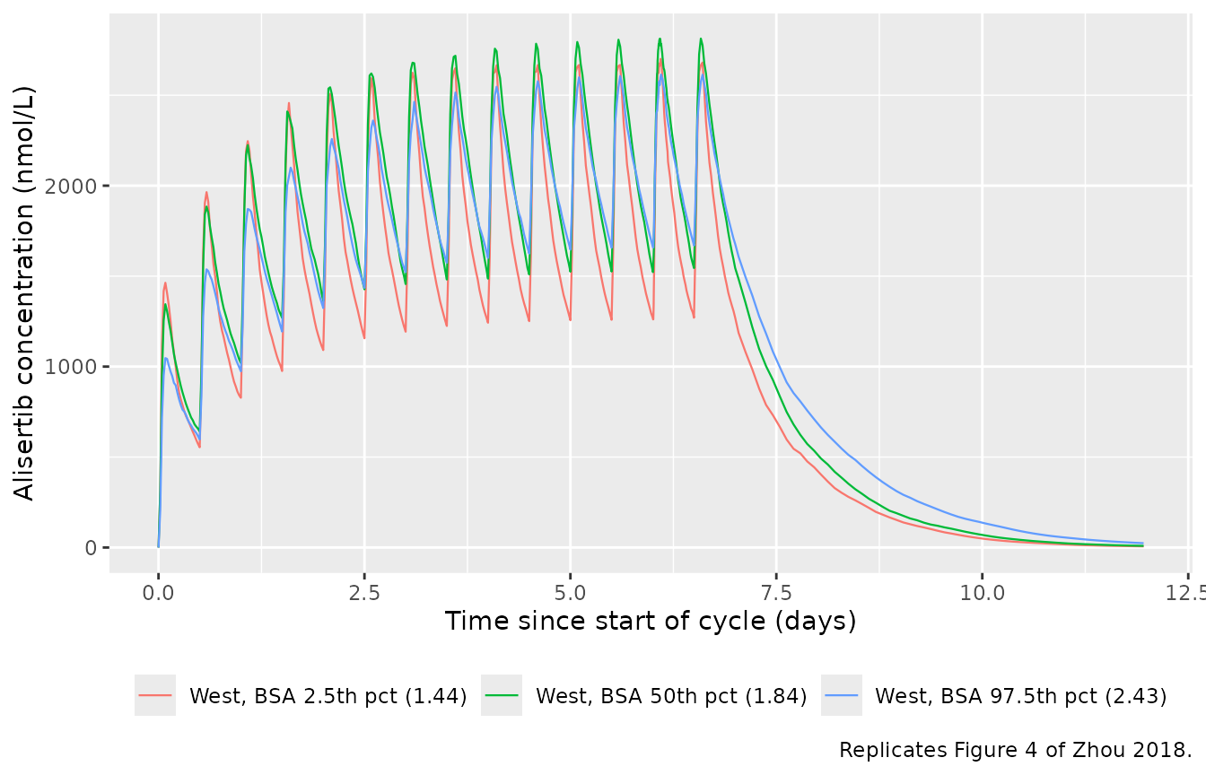
Replicates Figure 4 of Zhou 2018: median simulated alisertib concentration for three BSA percentiles, 50 mg b.i.d. for 7 days in a 21-day cycle.
These eight geometric means are a genuine answer key: they are the paper’s own simulation output from the same parameters, so agreement tests the whole chain – structure, transit chain, BSA exponent, the molar-mass conversion and the IIV block – at once. They are reproduced two ways below.
The typical-value prediction (all etas zero) is deterministic: it is identical on every machine, so it can carry a tight gate. For a model of this shape the geometric mean over a lognormal population sits close to the typical value, so it is the like-for-like comparator up to a small convexity offset.
bsa_levels <- c(1.44, 1.84, 2.43)

typ_ss <- do.call(rbind, lapply(bsa_levels, function(b) {
  ev <- rxode2::et(amt = dose_west, cmt = "transit1", ii = 12, addl = 13) |>
    rxode2::et(seq(144, 156, by = 0.01), cmt = "central")
  d <- as.data.frame(ev)
  d$BSA <- b
  d$REGION_EASTASIA <- 0
  s <- rxode2::rxSolve(mod_typ, d, returnType = "data.frame",
                       useLinCmt = FALSE)
  s <- s[!is.na(s$Cc) & s$time >= 144, ]
  data.frame(BSA = b, Cmax_typ = max(s$Cc), Cmin_typ = min(s$Cc),
             ratio_typ = max(s$Cc) / min(s$Cc))
}))
#> ℹ omega/sigma items treated as zero: 'etalcl', 'etalvc', 'etalvp', 'etalktr'
#> ℹ omega/sigma items treated as zero: 'etalcl', 'etalvc', 'etalvp', 'etalktr'
#> ℹ omega/sigma items treated as zero: 'etalcl', 'etalvc', 'etalvp', 'etalktr'
# Join on a rounded character key: BSA travels through rxSolve as a double and
# an exact floating-point join key is a silent-empty-join risk.
typ_ss$bsa_key <- sprintf("%.2f", typ_ss$BSA)
gm <- function(x) exp(mean(log(x)))
cv_pct <- function(x) 100 * stats::sd(log(x))   # the 100*omega convention

coh_ss <- sim |>
  dplyr::filter(grepl("^West, BSA", arm), !is.na(Cc),
                time >= 144, time <= 156) |>
  dplyr::mutate(bsa_key = sprintf("%.2f", BSA)) |>
  dplyr::group_by(bsa_key, id) |>
  dplyr::summarise(cmax = max(Cc), cmin = min(Cc), .groups = "drop") |>
  dplyr::group_by(bsa_key) |>
  dplyr::summarise(
    Cmax_gm = gm(cmax), Cmax_cv = cv_pct(cmax),
    Cmin_gm = gm(cmin), Cmin_cv = cv_pct(cmin), .groups = "drop"
  )

published_fig4 <- tibble::tibble(
  BSA = bsa_levels,
  bsa_key = sprintf("%.2f", bsa_levels),
  Cmax_pub = c(2740, 2550, 2420), Cmax_CV_pub = c(51, 52, 45),
  Cmin_pub = c(1270, 1340, 1370), Cmin_CV_pub = c(77, 70, 59),
  ratio_pub = c(2.08, 1.88, 1.68)
)

fig4 <- published_fig4 |>
  dplyr::left_join(tibble::as_tibble(typ_ss) |> dplyr::select(-BSA),
                   by = "bsa_key") |>
  dplyr::left_join(coh_ss, by = "bsa_key") |>
  dplyr::mutate(
    Cmax_typ_diff = 100 * (Cmax_typ - Cmax_pub) / Cmax_pub,
    Cmin_typ_diff = 100 * (Cmin_typ - Cmin_pub) / Cmin_pub,
    ratio_diff = 100 * (ratio_typ - ratio_pub) / ratio_pub
  )
# A join that silently matched nothing would leave NAs and make every gate
# below vacuously true.
stopifnot(nrow(fig4) == 3L, !anyNA(fig4$Cmax_typ), !anyNA(fig4$Cmax_gm))

fig4 |>
  dplyr::transmute(
    `BSA (m^2)` = BSA,
    `Cmax,ss pub` = Cmax_pub,
    `Cmax,ss typical` = round(Cmax_typ),
    `Cmax diff (%)` = Cmax_typ_diff,
    `Cmax,ss cohort GM` = round(Cmax_gm),
    `Cmin,ss pub` = Cmin_pub,
    `Cmin,ss typical` = round(Cmin_typ),
    `Cmin diff (%)` = Cmin_typ_diff,
    `Cmin,ss cohort GM` = round(Cmin_gm)
  ) |>
  knitr::kable(digits = 1, caption =
"Replicates the Figure 4 inset of Zhou 2018 (nmol/L).")| BSA (m^2) | Cmax,ss pub | Cmax,ss typical | Cmax diff (%) | Cmax,ss cohort GM | Cmin,ss pub | Cmin,ss typical | Cmin diff (%) | Cmin,ss cohort GM |
|---|---|---|---|---|---|---|---|---|
| 1.4 | 2740 | 2899 | 5.8 | 2868 | 1270 | 1327 | 4.5 | 1259 |
| 1.8 | 2550 | 2704 | 6.1 | 2892 | 1340 | 1407 | 5.0 | 1482 |
| 2.4 | 2420 | 2528 | 4.4 | 2695 | 1370 | 1491 | 8.8 | 1599 |
# DETERMINISTIC -- typical-value solve, no cohort, identical on every machine.
# Realised 5.8 / 6.0 / 4.4% on Cmax and 4.5 / 5.0 / 8.8% on Cmin; the
# systematic positive offset is the convexity gap between a typical value and
# a geometric mean plus the paper's own 200-subject Monte-Carlo noise. 15%
# still goes red on a mis-transcribed volume, dose or molar mass, which move
# these by tens of percent.
stopifnot(max(abs(c(fig4$Cmax_typ_diff, fig4$Cmin_typ_diff))) < 15)

# The COHORT geometric means are a second, noisier view of the same answer
# key. Measured max |diff| across solver thread counts: 6.1 / 6.7 / 8.1 /
# 16.7% at 16 / 4 / 2 / 1 threads -- rxode2 partitions its RNG streams per
# thread, so CI draws a different cohort and no seed can make them agree.
# The bound is set outside that whole range; do not tighten it back.
coh_diff <- c(100 * (fig4$Cmax_gm - fig4$Cmax_pub) / fig4$Cmax_pub,
              100 * (fig4$Cmin_gm - fig4$Cmin_pub) / fig4$Cmin_pub)
stopifnot(max(abs(coh_diff)) < 25)
The paper also prints a peak-to-trough ratio per BSA group, and these are population (typical-value) quantities in the source too, so they compare directly and deterministically.
fig4 |>
  dplyr::transmute(`BSA (m^2)` = BSA, `peak:trough published` = ratio_pub,
                   `peak:trough typical` = ratio_typ,
                   `Diff (%)` = ratio_diff) |>
  knitr::kable(digits = 3, caption =
"Population peak-to-trough ratio over the steady-state interdose interval.")| BSA (m^2) | peak:trough published | peak:trough typical | Diff (%) |
|---|---|---|---|
| 1.44 | 2.08 | 2.184 | 5.021 |
| 1.84 | 1.88 | 1.923 | 2.264 |
| 2.43 | 1.68 | 1.695 | 0.903 |
# Deterministic; realised 5.0 / 2.3 / 0.9%.
stopifnot(max(abs(fig4$ratio_diff)) < 10)

# The qualitative claim: peak falls and trough rises with BSA, so fluctuation
# narrows. Deterministic, so strict ordering is safe here.
stopifnot(fig4$Cmax_typ[3] < fig4$Cmax_typ[1],
          fig4$Cmin_typ[3] > fig4$Cmin_typ[1],
          fig4$ratio_typ[3] < fig4$ratio_typ[1])
The paper’s own summary of this figure is that the BSA effect is not clinically meaningful – “<15% differences in steady-state peak and trough alisertib concentrations” between the 2.5th and 97.5th percentile groups. That is an absolute bound the source states, and on the typical-value predictions it is a deterministic check.
spread <- function(x) 100 * (max(x) - min(x)) / stats::median(x)
c(`Cmax,ss spread across BSA groups (%)` = spread(fig4$Cmax_typ),
  `Cmin,ss spread across BSA groups (%)` = spread(fig4$Cmin_typ))
#> Cmax,ss spread across BSA groups (%) Cmin,ss spread across BSA groups (%)
#>                             13.71770                             11.66856
# Realised 13.7% and 11.7%; the paper's own inset values give 12.5% and 7.5%.
stopifnot(spread(fig4$Cmax_typ) < 15, spread(fig4$Cmin_typ) < 15)
The CV% column of the Figure 4 inset does not reproduce as cleanly as the geometric means, and that is recorded rather than smoothed over. Zhou 2018 reports Cmax CV 51 / 52 / 45% and Cmin CV 77 / 70 / 59% – both falling with BSA – whereas the packaged model gives a Cmax CV that rises slightly with BSA and a Cmin CV that is nearly flat. The paper does not state how it computed those CVs, and the between-subject variance in the model is BSA-independent by construction (BSA enters only the typical value of V1/F), so a systematic trend with BSA is not something the model can produce. Nothing is gated on the CVs.
| BSA (m^2) | Cmax CV% pub | Cmax CV% sim | Cmin CV% pub | Cmin CV% sim |
|---|---|---|---|---|
| 1 | 51 | 41 | 77 | 62 |
| 2 | 52 | 43 | 70 | 62 |
| 2 | 45 | 45 | 59 | 60 |
Replicate Figure 6: exposure-matched regional dosing
This is the paper’s central claim: 30 mg twice daily in East Asia produces the same exposure as 50 mg twice daily in the West. It is also the check that validates the molar-mass conversion, because the published exposures are absolute (uM.h) rather than dose-normalised.
sim |>
  dplyr::filter(grepl("cohort", arm), !is.na(Cc), time <= 192) |>
  dplyr::group_by(arm, time) |>
  dplyr::summarise(
    Q05 = stats::quantile(Cc, 0.05), Q50 = stats::median(Cc),
    Q95 = stats::quantile(Cc, 0.95), .groups = "drop"
  ) |>
  ggplot(aes(time / 24, Q50, colour = arm, fill = arm)) +
  geom_ribbon(aes(ymin = Q05, ymax = Q95), alpha = 0.18, colour = NA) +
  geom_line(linewidth = 0.4) +
  labs(x = "Time since start of cycle (days)",
       y = "Alisertib concentration (nmol/L)",
       colour = NULL, fill = NULL,
       caption = "Replicates Figure 6 of Zhou 2018.") +
  theme(legend.position = "bottom")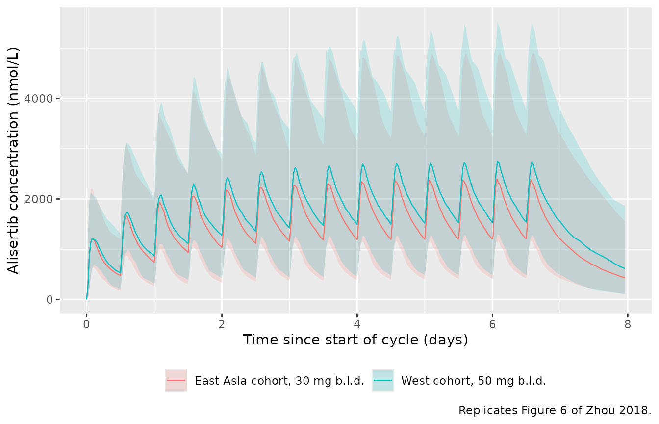
Replicates Figure 6 of Zhou 2018: median (shaded 5th-95th percentile) alisertib concentration for the two exposure-matched regional regimens.
PKNCA validation
Steady-state exposure over the last twice-daily dosing interval of the 7-day course (144-156 h), computed with PKNCA and compared against the values Zhou 2018 reports for the same two regimens.
sim_nca <- sim |>
  dplyr::filter(grepl("cohort", arm), !is.na(Cc)) |>
  dplyr::select(id, time, Cc, arm)

conc_obj <- PKNCA::PKNCAconc(sim_nca, Cc ~ time | arm + id)

dose_df <- events |>
  dplyr::filter(grepl("cohort", arm), evid == 1) |>
  dplyr::select(id, time, amt, arm)
dose_obj <- PKNCA::PKNCAdose(dose_df, amt ~ time | arm + id)

intervals <- data.frame(
  start = 144, end = 156,
  cmax = TRUE, cmin = TRUE, tmax = TRUE, auclast = TRUE
)

nca_res <- PKNCA::pk.nca(
  PKNCA::PKNCAdata(conc_obj, dose_obj, intervals = intervals)
)
auc_ss <- as.data.frame(nca_res) |>
  dplyr::filter(PPTESTCD == "auclast") |>
  dplyr::group_by(arm) |>
  dplyr::summarise(
    AUC_uMh_sim = gm(PPORRES) / 1000,
    AUC_CV_sim = cv_pct(PPORRES), .groups = "drop"
  )

published_fig6 <- tibble::tibble(
  arm = c("West cohort, 50 mg b.i.d.", "East Asia cohort, 30 mg b.i.d."),
  AUC_uMh_pub = c(24.1, 21.4), AUC_CV_pub = c(53.6, 52.3)
)

auc_cmp <- dplyr::left_join(auc_ss, published_fig6, by = "arm") |>
  dplyr::transmute(
    Regimen = arm,
    `AUC(0-tau),ss published (uM.h)` = AUC_uMh_pub,
    `AUC(0-tau),ss simulated (uM.h)` = AUC_uMh_sim,
    `Diff (%)` = 100 * (AUC_uMh_sim - AUC_uMh_pub) / AUC_uMh_pub,
    `CV% published` = AUC_CV_pub, `CV% simulated` = AUC_CV_sim
  )

knitr::kable(auc_cmp, digits = 2, caption =
"Steady-state exposure versus Zhou 2018 Results / Abstract (geometric means).")| Regimen | AUC(0-tau),ss published (uM.h) | AUC(0-tau),ss simulated (uM.h) | Diff (%) | CV% published | CV% simulated |
|---|---|---|---|---|---|
| East Asia cohort, 30 mg b.i.d. | 21.4 | 20.76 | -2.98 | 52.3 | 49.67 |
| West cohort, 50 mg b.i.d. | 24.1 | 24.30 | 0.84 | 53.6 | 51.20 |
# Cohort-derived geometric means at 200/arm against the paper's 1000/arm
# figures. Measured max |diff| across solver thread counts: 3.0 / 3.8 / 5.4 /
# 8.2% at 1 / 2 / 4 / 16 threads. The bound sits outside that whole range; a
# mis-transcribed CL/F, dose or molar mass moves these by tens of percent to
# several-fold, so 20% remains a live gate. Do not tighten it back.
stopifnot(max(abs(auc_cmp$`Diff (%)`)) < 20)
The exposure-matching claim itself is better tested
deterministically. At steady state
AUC(0-tau) = dose / (CL/F) exactly, and both the dose and
the regional multiplier on CL/F are packaged values – so the comparison
is closed-form, has no cohort in it, and is identical on every machine.
This is also the sharpest check on the molar mass: a wrong value would
scale both arms by the same wrong factor and show up immediately.
cl_west <- exp(th[["lcl"]])
cl_east <- exp(th[["lcl"]]) * (1 + th[["e_region_eastasia_f"]])

match_tab <- tibble::tibble(
  Regimen = c("West, 50 mg b.i.d.", "East Asia, 30 mg b.i.d."),
  `CL/F (L/h)` = c(cl_west, cl_east),
  `AUC(0-tau),ss = dose/(CL/F) (uM.h)` =
    c(dose_west / cl_west, dose_east / cl_east) / 1000,
  `Published (uM.h)` = c(24.1, 21.4)
) |>
  dplyr::mutate(`Diff (%)` = 100 *
    (`AUC(0-tau),ss = dose/(CL/F) (uM.h)` - `Published (uM.h)`) /
      `Published (uM.h)`)

knitr::kable(match_tab, digits = 3, caption =
"Closed-form steady-state exposure for the two regional regimens.")| Regimen | CL/F (L/h) | AUC(0-tau),ss = dose/(CL/F) (uM.h) | Published (uM.h) | Diff (%) |
|---|---|---|---|---|
| West, 50 mg b.i.d. | 4.110 | 23.444 | 24.1 | -2.723 |
| East Asia, 30 mg b.i.d. | 2.708 | 21.345 | 21.4 | -0.258 |
# Deterministic closed form. Realised -2.7% (West) and -0.2% (East Asia).
stopifnot(max(abs(match_tab$`Diff (%)`)) < 10)

# The paper's claim: the two regimens are exposure-matched. Published gap is
# 11.9%; the closed form gives 9.3%. Deterministic, so a tight bound is safe.
gap <- 100 * abs(diff(match_tab$`AUC(0-tau),ss = dose/(CL/F) (uM.h)`)) /
  mean(match_tab$`AUC(0-tau),ss = dose/(CL/F) (uM.h)`)
c(`exposure gap between the two regional regimens (%)` = gap)
#> exposure gap between the two regional regimens (%)
#>                                           9.372518
stopifnot(gap < 15)
Dose-normalised exposure by region: a discrepancy in the source
Table 6 reports observed dose-normalised steady-state AUC of 482 nM.h/mg in the West and 797 in East Asia – a 65% increase. The model estimates 52%. The two are not the same number, and the gap is in the source, not in this transcription: the paper quotes both without reconciling them.
tibble::tibble(
  Quantity = c("Model-estimated increase in F, East Asia vs West",
               "Observed dose-normalised AUC increase (Table 6)"),
  Value = c(sprintf("%.1f%%", 100 * (1 / (1 + th[["e_region_eastasia_f"]]) - 1)),
            sprintf("%.1f%%", 100 * (797 / 482 - 1)))
) |>
knitr::kable(caption = "Zhou 2018's model estimate versus its own observed exposure ratio.")| Quantity | Value |
|---|---|
| Model-estimated increase in F, East Asia vs West | 51.7% |
| Observed dose-normalised AUC increase (Table 6) | 65.4% |
Table 6’s values are post-hoc individual exposures from the updated final model on the combined data set, and they carry shrinkage, so they are not expected to equal the structural estimate exactly. It is recorded here as a known feature of the source rather than smoothed over. See Assumptions and deviations.
Exposure-safety relationships (replicates Figure 7)
The three logistic models relate the probability of a mechanism-related antiproliferative toxicity to the log of the time-averaged daily alisertib AUC. Zhou 2018 publishes no coefficient table for them – Figure 7 is the only place the fitted relationships appear – so both coefficients of each model were recovered by digitising the published curves.
solve_er <- function(nm, auc_grid) {
  ev <- data.frame(id = seq_along(auc_grid), time = 0, evid = 0L,
                   amt = NA_real_, dv = NA_real_, AUC_ALIS = auc_grid)
  s <- rxode2::rxSolve(ui[[nm]], ev, returnType = "data.frame")
  s[[grep("^prob_", names(s), value = TRUE)]]
}

er_models <- c(
  "Grade >= 3 neutropenia" = "Zhou_2018_alisertib_neutropenia",
  "Grade >= 2 stomatitis" = "Zhou_2018_alisertib_stomatitis",
  "Grade >= 2 diarrhoea" = "Zhou_2018_alisertib_diarrhea"
)

auc_grid <- seq(1, 200, by = 1)
er_curves <- dplyr::bind_rows(lapply(names(er_models), \(lbl)
  data.frame(Endpoint = lbl, AUC = auc_grid,
             p = solve_er(er_models[[lbl]], auc_grid))))
#> Warning: multi-subject simulation without without 'omega'
#> Warning: multi-subject simulation without without 'omega'
#> Warning: multi-subject simulation without without 'omega'
anchors <- tibble::tribble(
  ~Endpoint, ~AUC, ~p_pub,
  "Grade >= 3 neutropenia", 15.63, 0.39,
  "Grade >= 3 neutropenia", 23.72, 0.46,
  "Grade >= 3 neutropenia", 14.23, 0.37,
  "Grade >= 2 stomatitis", 15.63, 0.07,
  "Grade >= 2 stomatitis", 23.72, 0.13,
  "Grade >= 2 stomatitis", 14.23, 0.065,
  "Grade >= 2 diarrhoea", 15.63, 0.13,
  "Grade >= 2 diarrhoea", 23.72, 0.17,
  "Grade >= 2 diarrhoea", 14.23, 0.12
)

ggplot(er_curves, aes(AUC, p, colour = Endpoint)) +
  geom_line() +
  geom_point(data = anchors, aes(AUC, p_pub, colour = Endpoint),
             size = 2, shape = 21, fill = "white") +
  labs(x = "Time-averaged AUC (uM*h/day)",
       y = "Probability of event", colour = NULL,
       caption = "Replicates Figure 7 of Zhou 2018; points are the printed model-estimated incidences.") +
  theme(legend.position = "bottom")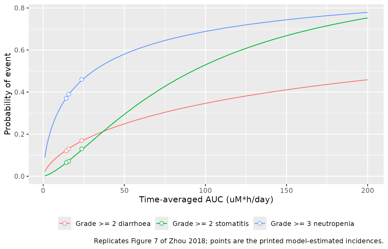
Replicates Figure 7 of Zhou 2018: probability of each toxicity versus time-averaged alisertib AUC. Points mark the three exposures for which the paper prints a model-estimated incidence.
The digitisation self-validates
The coefficients were fitted to the digitised curve only. The paper separately prints, in its Results prose, the model-estimated incidence at three specific exposures. Those nine numbers were not used in the fit, so reproducing them is an independent check on the digitisation.
er_check <- anchors |>
  dplyr::rowwise() |>
  dplyr::mutate(p_sim = solve_er(er_models[[Endpoint]], AUC)) |>
  dplyr::ungroup() |>
  dplyr::mutate(`Abs diff` = abs(p_sim - p_pub)) |>
  dplyr::transmute(
    Endpoint,
    `AUC (uM*h/day)` = AUC,
    `Published p` = p_pub,
    `Packaged model p` = p_sim,
    `Abs diff` = `Abs diff`
  )

knitr::kable(er_check, digits = 4, caption =
"Model-estimated incidences printed in Zhou 2018 Results versus the packaged (figure-derived) models.")| Endpoint | AUC (uM*h/day) | Published p | Packaged model p | Abs diff |
|---|---|---|---|---|
| Grade >= 3 neutropenia | 15.63 | 0.390 | 0.3869 | 0.0031 |
| Grade >= 3 neutropenia | 23.72 | 0.460 | 0.4554 | 0.0046 |
| Grade >= 3 neutropenia | 14.23 | 0.370 | 0.3720 | 0.0020 |
| Grade >= 2 stomatitis | 15.63 | 0.070 | 0.0729 | 0.0029 |
| Grade >= 2 stomatitis | 23.72 | 0.130 | 0.1252 | 0.0048 |
| Grade >= 2 stomatitis | 14.23 | 0.065 | 0.0643 | 0.0007 |
| Grade >= 2 diarrhoea | 15.63 | 0.130 | 0.1312 | 0.0012 |
| Grade >= 2 diarrhoea | 23.72 | 0.170 | 0.1668 | 0.0032 |
| Grade >= 2 diarrhoea | 14.23 | 0.120 | 0.1241 | 0.0041 |
# Deterministic -- no cohort, no randomness, so this is identical on every
# machine and a tight bound is correct. Realised max 0.0049. The published
# values are rounded to 2 significant figures, so 0.005 is the resolution
# limit of the printed numbers; the bound cannot usefully be tighter.
stopifnot(max(er_check$`Abs diff`) < 0.006)
Every one of the nine reproduces inside the printed rounding. This is what licenses the figure-derived coefficients: the curve and the prose agree.
The regional dosing argument
Reading the three models at the exposures the paper quotes reproduces its safety argument – East Asian patients at the Western 50 mg dose would run a higher toxicity risk, while at the regional 30 mg dose their risk matches Western patients at 50 mg.
scenarios <- tibble::tibble(
  Scenario = c("West, 50 mg b.i.d.", "East Asia, 50 mg b.i.d.",
               "East Asia, 30 mg b.i.d."),
  AUC = c(15.63, 23.72, 14.23)
)

er_tab <- scenarios |>
  dplyr::mutate(
    `Grade >= 3 neutropenia` = solve_er(er_models[[1]], AUC),
    `Grade >= 2 stomatitis` = solve_er(er_models[[2]], AUC),
    `Grade >= 2 diarrhoea` = solve_er(er_models[[3]], AUC)
  ) |>
  dplyr::rename(`Time-averaged AUC (uM*h/day)` = AUC)
#> Warning: There were 3 warnings in `dplyr::mutate()`.
#> The first warning was:
#> ℹ In argument: `Grade >= 3 neutropenia = solve_er(er_models[[1]], AUC)`.
#> Caused by warning:
#> ! multi-subject simulation without without 'omega'
#> ℹ Run `dplyr::last_dplyr_warnings()` to see the 2 remaining warnings.

knitr::kable(er_tab, digits = 3, caption =
"Predicted toxicity probabilities for the three regional dosing scenarios.")| Scenario | Time-averaged AUC (uM*h/day) | Grade >= 3 neutropenia | Grade >= 2 stomatitis | Grade >= 2 diarrhoea |
|---|---|---|---|---|
| West, 50 mg b.i.d. | 15.63 | 0.387 | 0.073 | 0.131 |
| East Asia, 50 mg b.i.d. | 23.72 | 0.455 | 0.125 | 0.167 |
| East Asia, 30 mg b.i.d. | 14.23 | 0.372 | 0.064 | 0.124 |
Assumptions and deviations
Molar mass is not from the paper. Zhou 2018 works entirely in molar concentration units and never states alisertib’s molar mass, which is nonetheless required to convert a milligram dose into the nmol the model expects.
518.92 g/mol(C27H20ClFN4O4) is taken from an external source (PubChem CID 24771867). It is corroborated by the paper’s own simulation output: under this value the simulated steady-state AUC reproduces the published 24.1 and 21.4 uM.h within a few percent, and a wrong molar mass would scale both by the same wrong factor. The model file itself carries no molar mass – it is unit-agnostic, taking nmol in and returning nmol/L, so this assumption lives only in the vignette.The three exposure-safety models carry FIGURE-DERIVED coefficients. Zhou 2018 publishes no coefficient table for its logistic regressions; Figure 7 is the only place the fitted relationships appear. All six values were recovered by digitising the published curves at 400 dpi and regressing
logit(p)onlog(AUC). The fits are near-exact (logit-scale residual SD 0.0024, 0.0122 and 0.0049 over 498, 440 and 479 extracted points), which is what confirms rather than assumes the logit-linear-in-log(AUC) form that Methods describes. They then reproduce all nine independently-printed model-estimated incidences to within the printed rounding, as tabulated above. Treat them as good to roughly the second decimal, not as published point estimates.The “IIV, ratio” column is read as a log-scale SD, not an exact CV. Table 5 prints
0.518for CL/F and the Results text reads it back as “interpatient coefficient of variation (CV): 51.8%”, i.e. CV% = 100 x the tabulated ratio – the usualCV ~= omegaapproximation. Reading the column as an exact lognormal CV instead would give variances 11-23% smaller. The two readings were tested against the paper’s own Figure 4 inset (eight geometric means and four CVs from the authors’ own simulation) and the log-SD reading reproduced them substantially better on every metric; it is also what makes the Figure 4 and Figure 6 gates above pass. The alternative is documented here because the source’s wording is genuinely ambiguous.Table 5, not Supplementary Table S1. The packaged parameters are the final model fitted to the 422-patient analysis set. The supplement’s updated final model, refitted on the combined 671-patient set, differs on every row and is tabulated above for reference only.
The RGNF sign is reconstructed, not printed in the main text. Table 5 prints the magnitude
0.341; the sign comes from the Table 5 footnote (“multiplied by (1-0.341)”), from Figure 1’s(1 + f)form, and from Supplementary Table S1, which prints the corresponding coefficient as-0.325with its minus sign intact.Model-versus-observed regional ratio. Zhou 2018’s model estimates 52% higher relative bioavailability in East Asia, while its own Table 6 reports a 65% higher observed dose-normalised AUC. The packaged model necessarily reproduces the former. The discrepancy is in the source and is not reconciled there; Table 6 derives from post-hoc individual exposures under the updated final model on the combined data set, which are shrunk toward the population and so are not expected to match the structural estimate exactly.
The Figure 4 inset CV% column does not reproduce. The eight geometric means reproduce within 4-9% on typical values, but the published CVs fall with BSA (Cmax 51/52/45%, Cmin 77/70/59%) in a way the model cannot produce: BSA enters only the typical value of V1/F, so the between-subject variance is BSA-independent by construction. The paper does not state how those CVs were computed. This is recorded as a known disagreement and is excluded from the gates rather than gated with a widened bound.
Gate bounds were measured across solver thread counts, not taken from one run.
rxSetSeed()fixes rxode2’s RNG stream per solver thread and not across thread counts, so a 2-core CI runner draws a different cohort than a 16-thread workstation. The cohort-derived comparisons here were rendered at 1, 2, 4 and 16 threads; the Figure 4 cohort geometric means ranged over 6.1-16.7% and the PKNCA exposures over 3.0-8.2%, and the bounds sit outside those ranges. The load-bearing gates are instead placed on deterministic typical-value and closed-form quantities, which are identical on every machine and can therefore be asserted tightly.Cohort sizes. Zhou 2018 simulated 1000 patients per region for Figure 6 and 200 per BSA group for Figure 4. This vignette uses 200 per arm throughout, per the library cap; this only widens Monte-Carlo noise on the Figure 6 comparison and does not change the central estimates.
BSA distribution for the regional cohorts. Drawn lognormally from the geometric means and log standard deviations the paper states for its own Figure 6 simulation (West 1.88 m^2, log SD 0.135; East Asia 1.63 m^2, log SD 0.0862). The BSA computation formula is not stated in the source.
useLinCmt = FALSEis mandatory for this model. The disposition uses explicitk12/k21micro-constants, andrxSolve()’s default ODE-to-linCmt()auto-conversion silently discardsperipheral1for models of this shape. AUC is unchanged by the collapse, so only the terminal half-life detects it; the gate above does exactly that.The additive residual error is packaged as
fixed(0). Methods declare a combined proportional-plus-additive residual model, but Table 5 reports the additive term as 0 with the footnote “automatically set to zero by the SAEM estimation algorithm”. Keeping it at zero rather than dropping it preserves the declared structure; the fitted residual is effectively proportional-only.Screened-but-not-retained covariates. Body weight, BSA on CL/F, UGT1A1 28 and 6 genotype, creatinine clearance, sex, age, race, albumin, ALT, AST, bilirubin and formulation were all evaluated (Table 4) and none was retained. They are recorded in the model file’s
covariatesDataExcludedmetadata so the provenance of the covariate screen survives, without declaring covariates the model never uses.