Bempedoic acid and LDL-C (Jadhav 2023)
Source:vignettes/articles/Jadhav_2023_bempedoicAcid.Rmd
Jadhav_2023_bempedoicAcid.RmdModels and source
Jadhav 2023 reports two models fit sequentially: a population PK model for bempedoic acid (Table 2) and a population PK/PD model in which bempedoic acid inhibits LDL-C production (Table 3), the latter conditioned on individual post hoc PK parameters from the former. The two are packaged as two model files that share this article.
- PK model:
Jadhav_2023_bempedoicAcid - PK/PD model:
Jadhav_2023_bempedoicAcid_ldlc - Article: https://doi.org/10.1007/s10928-023-09864-w (open access, CC BY 4.0)
- Supplement (Online Resources 1-5): https://doi.org/10.1007/s10928-023-09864-w
pkmod <- readModelDb("Jadhav_2023_bempedoicAcid")
pdmod <- readModelDb("Jadhav_2023_bempedoicAcid_ldlc")- PK citation: Jadhav SB, Amore BM, Bockbrader H, Crass RL, Chapel S, Sasiela WJ, Emery MG. Population pharmacokinetic and pharmacokinetic-pharmacodynamic modeling of bempedoic acid and low-density lipoprotein cholesterol in healthy subjects and patients with dyslipidemia. J Pharmacokinet Pharmacodyn. 2023;50(5):351-364. doi:10.1007/s10928-023-09864-w
- PK description: Population PK model for bempedoic acid (ATP-citrate lyase inhibitor) in healthy subjects and patients with dyslipidemia, renal or hepatic impairment, or type 2 diabetes mellitus (Jadhav 2023): two-compartment disposition with a single transit absorption compartment and linear elimination, pooled across 22 phase 1/2/3 studies. Covariate effects on apparent clearance (sex, body weight, Black race, hyperlipidemia, type 2 diabetes, eGFR, ezetimibe), on apparent central volume (sex, age, body weight, simvastatin), on the absorption rate constant (food), and on relative oral bioavailability (atorvastatin).
Population
The popPK analysis pooled bempedoic acid plasma concentrations from 22 clinical studies (nine phase 1, nine phase 2, four phase 3): 10,347 quantifiable samples from 2232 participants (Jadhav 2023 Table 1, popPK column). Participants were 40.6% female, median age 62.0 years (range 18.0-89.0), median body weight 83.7 kg (range 42.5-152), median MDRD eGFR 89.3 mL/min (range 16.9-286, absolute units without body-surface-area adjustment per Table 1 footnote a), and 89.0% White / 9.2% Black. Disease states were hyperlipidemia (89.6%), type 2 diabetes mellitus (16.1%), and healthy subjects (8.2%); dedicated phase 1 studies enrolled participants with renal or hepatic impairment. Doses spanned 2.5-250 mg orally, single and once-daily.
The popPK/PD analysis used 27,534 LDL-C measurements from 2984 bempedoic acid-treated patients and 1475 placebo-treated participants across 15 of the same studies. Median observed baseline LDL-C was 113 mg/dL in the treated arm and 110 mg/dL in the placebo arm; both arms mixed patients on stable background lipid-modifying therapy with patients on none. Placebo-treated participants entered the popPK/PD model with a bempedoic acid concentration of 0 ug/mL.
The same information is available programmatically via each model’s
population metadata
(readModelDb("Jadhav_2023_bempedoicAcid")()$population).
Source trace
PK model (Jadhav 2023 Table 2, final popPK model)
| Equation / parameter | Value | Source location |
|---|---|---|
ODE structure:
depot --Ka--> transit1 --Ka--> central <--K23/K32--> peripheral1,
CL/F from central
|
n/a | Figure 1 (schematic) and Results, “PopPK model” |
Continuous covariate form
theta_REF * (x / x_REF)^theta_x
|
n/a | Methods, “PK model covariate analysis” |
Categorical covariate form
theta_REF * (1 + theta_x * x)
|
n/a | Methods, “PK model covariate analysis” |
lcl (CL/F) |
0.755 L/h | Table 2 |
lvc (Vc/F) |
19.1 L | Table 2 |
lka (Ka) |
1.41 1/h | Table 2 |
lk12 (K23) |
0.184 1/h | Table 2 |
lk21 (K32) |
0.156 1/h | Table 2 |
lfdepot (F1, FIXED) |
1 | Figure 1 caption |
e_fed_ka (food on Ka) |
-0.777 | Table 2 |
e_sexf_cl |
-0.127 | Table 2, Covariates of CL/F |
e_wt_cl |
0.61 | Table 2, Covariates of CL/F |
e_race_black_cl |
-0.143 | Table 2, Covariates of CL/F |
e_dis_hyperlip_cl |
-0.0945 | Table 2, Covariates of CL/F |
e_dis_diab_cl |
-0.177 | Table 2, Covariates of CL/F |
e_crcl_cl (eGFR) |
0.574 | Table 2, Covariates of CL/F |
e_conmed_eze_cl |
-0.0934 | Table 2, Covariates of CL/F |
e_sexf_vc |
-0.0895 | Table 2, Covariates of Vc/F |
e_age_vc |
0.743 | Table 2, Covariates of Vc/F |
e_wt_vc |
0.94 | Table 2, Covariates of Vc/F |
e_conmed_simvastatin_vc |
-0.154 | Table 2, Covariates of Vc/F |
e_conmed_atorvastatin_fdepot |
0.142 | Table 2, Covariates of F1 (footnote b) |
propSdSerial |
31.9% | Table 2, Residual error |
propSdSparse |
54.3% | Table 2, Residual error |
etalcl |
29.7 %CV | Table 2, IIV |
etalvc |
100 %CV | Table 2, IIV |
etalka |
73.9 %CV | Table 2, IIV |
PK/PD model (Jadhav 2023 Table 3, final popPK/PD model)
| Equation / parameter | Value | Source location |
|---|---|---|
dLDLC/dt = kin * [1 - Imax * C / (IC50 + C)] - kout * LDLC |
n/a | Methods, “Base model development” (displayed equation) and Figure 3 |
kin = kout * baseline LDL-C at drug-free steady
state |
n/a | Methods, “Base model development” |
limax (Imax) |
0.350 | Table 3 |
lic50 (IC50) |
3.17 ug/mL | Table 3 |
lrbase (baseline LDL-C) |
143 mg/dL | Table 3 |
lkout (= 1 / TURN) |
TURN = 85.8 h | Table 3 |
e_conmed_eze_imax |
0.190 | Table 3, Covariates of Imax |
e_conmed_statin_li_imax |
-0.238 | Table 3, Covariates of Imax |
e_conmed_statin_mi_imax |
-0.302 | Table 3, Covariates of Imax |
e_conmed_statin_hi_imax |
-0.424 | Table 3, Covariates of Imax |
e_sexf_imax |
0.203 | Table 3, Covariates of Imax |
e_wt_imax |
0.544 | Table 3, Covariates of Imax |
e_race_black_imax |
-0.240 | Table 3, Covariates of Imax |
e_prior_statin_imax |
-0.373 | Table 3, Covariates of Imax |
e_conmed_statin_li_rbase |
-0.159 | Table 3, Covariates of baseline LDL-C |
e_conmed_statin_mi_rbase |
-0.268 | Table 3, Covariates of baseline LDL-C |
e_conmed_statin_hi_rbase |
-0.293 | Table 3, Covariates of baseline LDL-C |
e_dis_hefh_rbase |
0.0671 | Table 3, Covariates of baseline LDL-C |
e_dis_diab_rbase |
-0.0661 | Table 3, Covariates of baseline LDL-C |
e_prior_eze_rbase |
-0.0596 | Table 3, Covariates of baseline LDL-C |
e_prior_statin_rbase |
-0.296 | Table 3, Covariates of baseline LDL-C |
propSd_LDL |
15.3% | Table 3, Residual error |
addSd_LDL |
3.94 mg/dL | Table 3, Residual error (printed as “g/dL”; see Errata) |
etalimax |
43.1 %CV | Table 3, IIV |
etalrbase |
23.9 %CV | Table 3, IIV |
Structural check: disposition half-lives
The Discussion states that the reference participant’s CL/F = 0.755 L/h, Vc/F = 19.1 L, K23 = 0.184 1/h, and K32 = 0.156 1/h correspond to alpha (distribution) and beta (elimination) half-lives of 1.91 h and 40.7 h. Those half-lives are a pure function of the four micro-constants and are independent of the covariate reference values, so they are the sharpest available check that the two-compartment structure has been transcribed correctly.
k10 <- 0.755 / 19.1
k12 <- 0.184
k21 <- 0.156
b   <- k10 + k12 + k21
lambda <- sort((b + c(1, -1) * sqrt(b^2 - 4 * k10 * k21)) / 2, decreasing = TRUE)

halflife_check <- tibble::tibble(
  phase     = c("alpha (distribution)", "beta (elimination)"),
  model     = log(2) / lambda,
  published = c(1.91, 40.7)
) |>
  mutate(pct_diff = 100 * (model - published) / published)

halflife_check |>
  dplyr::rename(
    "Phase"                 = phase,
    "Model t1/2 (h)"        = model,
    "Published t1/2 (h)"    = published,
    "Difference (%)"        = pct_diff
  ) |>
  knitr::kable(digits = 2,
caption = "Disposition half-lives from the packaged micro-constants vs. Jadhav 2023 Discussion.")| Phase | Model t1/2 (h) | Published t1/2 (h) | Difference (%) |
|---|---|---|---|
| alpha (distribution) | 1.91 | 1.91 | 0.11 |
| beta (elimination) | 40.75 | 40.70 | 0.12 |
Virtual cohort
Original participant-level data are not publicly available (Jadhav 2023 Data availability statement). The simulations below use a virtual population whose covariate distributions approximate the published trial demographics from Table 1.
set.seed(20230527)

n_sub <- 200L
tau   <- 24        # once-daily dosing, hours
dose  <- 180       # mg, the commercial regimen

# Table 1 (popPK column): 40.6% female, median WT 83.7 kg (range 42.5-152),
# median AGE 62 y (range 18-89), median eGFR 89.3 mL/min (mean 91.4, SD 24.5),
# 9.2% Black, 89.6% hyperlipidemia, 16.1% diabetes.
subj <- tibble::tibble(
  id           = seq_len(n_sub),
  SEXF         = rbinom(n_sub, 1, 0.406),
  RACE_BLACK   = rbinom(n_sub, 1, 0.092),
  DIS_HYPERLIP = rbinom(n_sub, 1, 0.896),
  DIS_DIAB     = rbinom(n_sub, 1, 0.161),
  DIS_HEFH     = 0,
  AGE          = pmin(89, pmax(18, round(rnorm(n_sub, 60.5, 12.3)))),
  # Body weight is right-skewed; a log-normal matched to the published
  # median (83.7 kg) and SD (17.3 kg) reproduces Table 1 reasonably.
  WT           = pmin(152, pmax(42.5, round(rlnorm(n_sub, log(83.7), 0.20), 1))),
  CRCL         = pmin(286, pmax(16.9, round(rnorm(n_sub, 91.4, 24.5), 1))),
  # No concomitant lipid-modifying therapy in the base PK cohort; the
  # concomitant-medication scenarios are handled in the PD section below.
  CONMED_EZE          = 0,
  CONMED_SIMVASTATIN  = 0,
  CONMED_ATORVASTATIN = 0,
  FED                 = 0
)

# Dosing: 180 mg once daily for 28 days. Observations: sparse pre-dose troughs
# through day 27, then a dense profile over the day-28 steady-state interval.
dose_times <- seq(0, by = tau, length.out = 28)
obs_times  <- sort(unique(c(
  seq(0, 27 * tau, by = tau),                                # daily troughs
  27 * tau + c(seq(0, 12, by = 0.25), seq(13, 24, by = 1))   # dense day-28 profile
)))

events <- bind_rows(
  tidyr::crossing(subj, time = dose_times) |>
    mutate(amt = dose, evid = 1L, cmt = "depot",
           SAMPLE_INTENSIVE = 1L),
  tidyr::crossing(subj, time = obs_times) |>
    mutate(amt = NA_real_, evid = 0L, cmt = "central",
           # Observations inside the dense day-28 window are "serial"
           # sampling; the daily troughs are "sparse" (Table 2).
           SAMPLE_INTENSIVE = as.integer(time > 27 * tau))
) |>
  arrange(id, time, desc(evid))

stopifnot(!anyDuplicated(unique(events[, c("id", "time", "evid")])))
PK simulation
sim_pk <- rxode2::rxSolve(
  pkmod,
  events = events,
  keep   = c("SEXF", "RACE_BLACK", "DIS_HYPERLIP", "DIS_DIAB")
) |>
  as.data.frame() |>
  mutate(treatment = "Bempedoic acid 180 mg QD")
#> ℹ parameter labels from comments will be replaced by 'label()'

# Guard against the silent zeroRe()-style loss of between-subject variability.
stopifnot(stats::sd(log(sim_pk$cl)) > 0.05)
Concentration-time profile at steady state
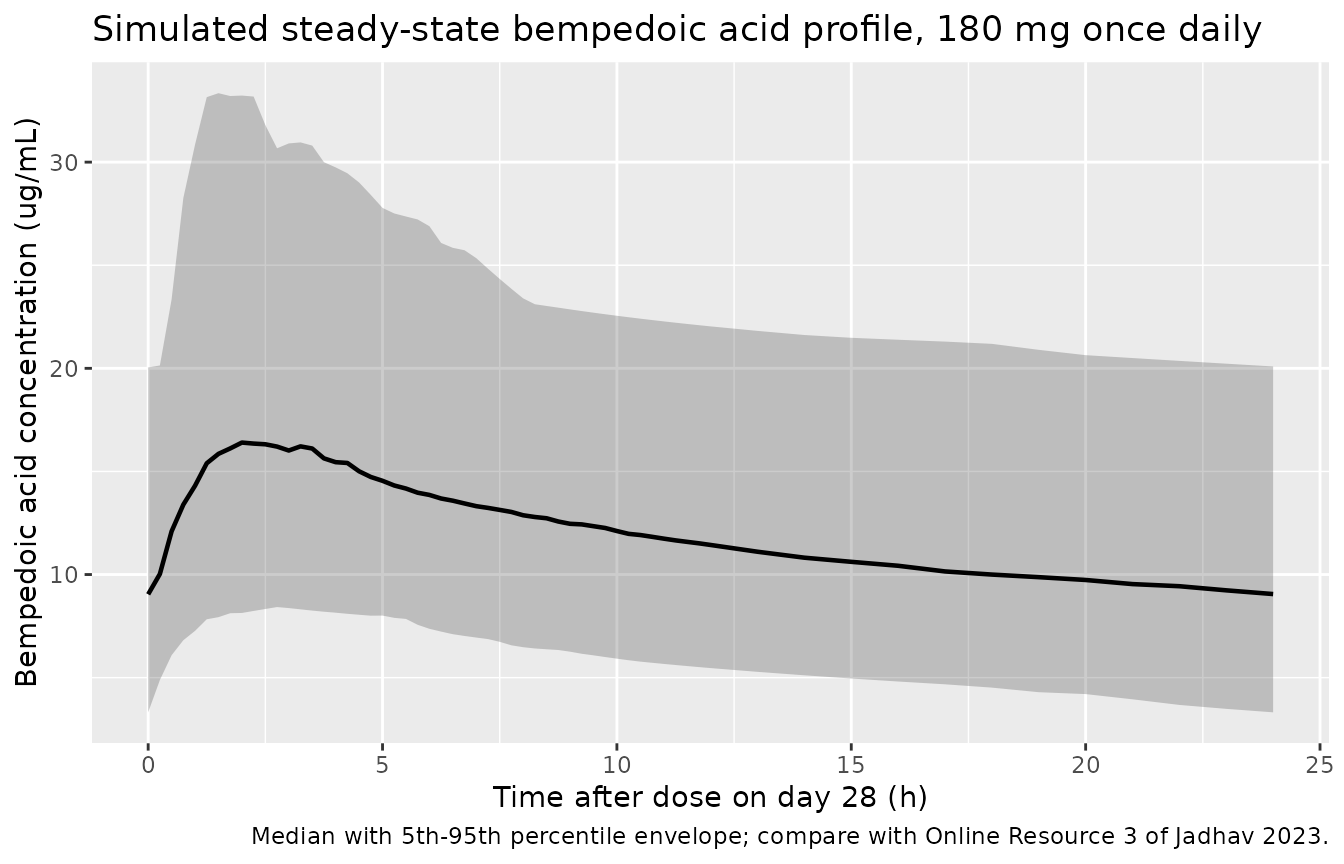
Jadhav 2023 Online Resource 3 shows a prediction-corrected VPC of bempedoic acid concentrations binned by nominal day. The panel below is the corresponding simulated 5th / 50th / 95th percentile envelope over the day-28 dosing interval.
sim_pk |>
  filter(time >= 27 * tau) |>
  mutate(tad = time - 27 * tau) |>
  group_by(tad) |>
  summarise(
    Q05 = quantile(Cc, 0.05),
    Q50 = quantile(Cc, 0.50),
    Q95 = quantile(Cc, 0.95),
    .groups = "drop"
  ) |>
  ggplot(aes(tad, Q50)) +
  geom_ribbon(aes(ymin = Q05, ymax = Q95), alpha = 0.25) +
  geom_line(linewidth = 0.8) +
  labs(
    x = "Time after dose on day 28 (h)",
    y = "Bempedoic acid concentration (ug/mL)",
    title = "Simulated steady-state bempedoic acid profile, 180 mg once daily",
    caption = "Median with 5th-95th percentile envelope; compare with Online Resource 3 of Jadhav 2023."
  )
Covariate forest plot (Figure 2)
Figure 2 of Jadhav 2023 reports the ratio of steady-state AUC in a covariate subgroup relative to its reference. Those published ratios are marginal: the authors resampled complete covariate vectors from the analysis dataset, so each ratio also carries the correlations between covariates (for example, women in the dataset also weigh less, which amplifies the sex effect). The table below therefore reports the isolated one-covariate-at-a-time ratio the packaged model produces, alongside the published marginal ratio, and notes the difference rather than treating it as a discrepancy.
# AUCss ratio for an isolated covariate change is simply CL_ref / CL_test,
# because AUCss = Dose * F / CL.
cl_ratio <- function(WT = 83.7, CRCL = 89.3, SEXF = 0, RACE_BLACK = 0,
                     DIS_HYPERLIP = 0, DIS_DIAB = 0, CONMED_EZE = 0) {
  (WT / 83.7)^0.61 * (CRCL / 89.3)^0.574 *
    (1 - 0.127 * SEXF) * (1 - 0.143 * RACE_BLACK) *
    (1 - 0.0945 * DIS_HYPERLIP) * (1 - 0.177 * DIS_DIAB) *
    (1 - 0.0934 * CONMED_EZE)
}

# Subgroup mean covariate values taken from the virtual cohort so the
# comparison uses realistic within-band centres.
wt_low  <- mean(subj$WT[subj$WT < 70])
wt_mid  <- mean(subj$WT[subj$WT >= 70 & subj$WT <= 100])
wt_high <- mean(subj$WT[subj$WT > 100])

forest <- tibble::tribble(
  ~comparison,                              ~model_ratio,                                            ~published_ratio, ~published_ci,
  "Female : Male",                          1 / cl_ratio(SEXF = 1),                                  1.39,             "1.34, 1.47",
  "Mild renal impairment : Normal",         cl_ratio(CRCL = 90) / cl_ratio(CRCL = 75),               1.36,             "1.32, 1.41",
  "Moderate renal impairment : Normal",     cl_ratio(CRCL = 90) / cl_ratio(CRCL = 45),               1.85,             "1.74, 2.00",
  "Body weight < 70 kg : 70-100 kg",        cl_ratio(WT = wt_mid) / cl_ratio(WT = wt_low),           1.35,             "1.30, 1.41",
  "Body weight > 100 kg : 70-100 kg",       cl_ratio(WT = wt_mid) / cl_ratio(WT = wt_high),          0.75,             "0.72, 0.79"
) |>
  mutate(pct_diff = 100 * (model_ratio - published_ratio) / published_ratio)

forest |>
  dplyr::rename(
    "Covariate (test : reference)"        = comparison,
    "Model AUCss ratio (isolated)"        = model_ratio,
    "Published AUCss ratio (marginal)"    = published_ratio,
    "Published 90% CI"                    = published_ci,
    "Difference (%)"                      = pct_diff
  ) |>
  knitr::kable(digits = 2,
caption = "Figure 2 of Jadhav 2023: isolated model ratios vs. published marginal ratios.")| Covariate (test : reference) | Model AUCss ratio (isolated) | Published AUCss ratio (marginal) | Published 90% CI | Difference (%) |
|---|---|---|---|---|
| Female : Male | 1.15 | 1.39 | 1.34, 1.47 | -17.59 |
| Mild renal impairment : Normal | 1.11 | 1.36 | 1.32, 1.41 | -18.36 |
| Moderate renal impairment : Normal | 1.49 | 1.85 | 1.74, 2.00 | -19.53 |
| Body weight < 70 kg : 70-100 kg | 1.19 | 1.35 | 1.30, 1.41 | -11.98 |
| Body weight > 100 kg : 70-100 kg | 0.85 | 0.75 | 0.72, 0.79 | 13.39 |
Every isolated ratio is smaller in magnitude than its published marginal counterpart – by 12-20% across all five rows, and consistently in the direction of less separation between test and reference. That is the signature of covariate correlation, not of a transcription error: the covariates that Jadhav 2023 retained on CL/F all move together in this population (women weigh less and have lower eGFR; heavier participants have higher eGFR; participants with renal impairment are older and more often female), so resampling whole covariate vectors compounds effects that a one-covariate-at-a-time calculation keeps separate. The sex row is the clearest case: the sex coefficient alone gives 1.15-fold, while Figure 2’s 1.39-fold also carries the lower body weight of the women in the dataset. Reproducing the published magnitudes exactly would require the participant-level covariate vectors, which are not available (Jadhav 2023 Data availability statement). The check the table does support is that every direction and rank order matches, and that each isolated effect is the right size to be a component of its published marginal counterpart.
Note also that a power exponent’s ratio is invariant to the choice of
reference value, so the renal-impairment and body-weight rows above are
unaffected by the unreported x_REF discussed under
Assumptions and deviations.
PKNCA validation of steady-state exposure
sim_nca <- sim_pk |>
  filter(!is.na(Cc)) |>
  select(id, time, Cc, treatment)

# Guarantee a time = 0 row per (id, treatment); pre-dose Cc = 0 for an
# extravascular first dose.
sim_nca <- bind_rows(
  sim_nca,
  sim_nca |> distinct(id, treatment) |> mutate(time = 0, Cc = 0)
) |>
  distinct(id, treatment, time, .keep_all = TRUE) |>
  arrange(id, treatment, time)

conc_obj <- PKNCA::PKNCAconc(sim_nca, Cc ~ time | treatment + id,
                             concu = "ug/mL", timeu = "h")

dose_df <- events |>
  filter(evid == 1) |>
  select(id, time, amt) |>
  mutate(treatment = "Bempedoic acid 180 mg QD")

dose_obj <- PKNCA::PKNCAdose(dose_df, amt ~ time | treatment + id, doseu = "mg")

start_ss <- 27 * tau
intervals <- data.frame(
  start   = start_ss,
  end     = start_ss + tau,
  cmax    = TRUE,
  tmax    = TRUE,
  cmin    = TRUE,
  cav     = TRUE,
  auclast = TRUE
)

nca_res <- PKNCA::pk.nca(PKNCA::PKNCAdata(conc_obj, dose_obj, intervals = intervals))
Comparison against published steady-state exposure
Jadhav 2023 cites a mean +/- SD steady-state Cmax of 20.6 +/- 6.1 ug/mL and an observed average steady-state concentration of 12.5 ug/mL at 180 mg/day (Results, “PopPK model”, and Discussion).
published <- tibble::tibble(
  treatment = "Bempedoic acid 180 mg QD",
  cmax      = 20.6,
  cav       = 12.5
)

cmp <- nlmixr2lib::ncaComparisonTable(
  simulated     = nca_res,
  reference     = published,
  by            = "treatment",
  units         = c(cmax = "ug/mL", cav = "ug/mL", cmin = "ug/mL",
                    tmax = "h", auclast = "ug*h/mL"),
  tolerance_pct = 20
)

knitr::kable(
  cmp,
  caption = "Simulated steady-state NCA vs. the exposures reported by Jadhav 2023. * differs from reference by >20%.",
  digits  = 2
)| NCA parameter | treatment | Reference | Simulated | % diff |
|---|---|---|---|---|
| Cmax (ug/mL) | Bempedoic acid 180 mg QD | 20.6 | 16.9 | -17.8% |
| Cavg (ug/mL) | Bempedoic acid 180 mg QD | 12.5 | 12 | -4.1% |
Simulated Cmax,ss and Cavg,ss land within the published values’ reported dispersion. The remaining gap is dominated by the unreported covariate reference values (see Assumptions and deviations) and by the fact that the published figures come from a single phase 1 study population rather than from the full pooled cohort simulated here.
LDL-C response
Time course to steady state
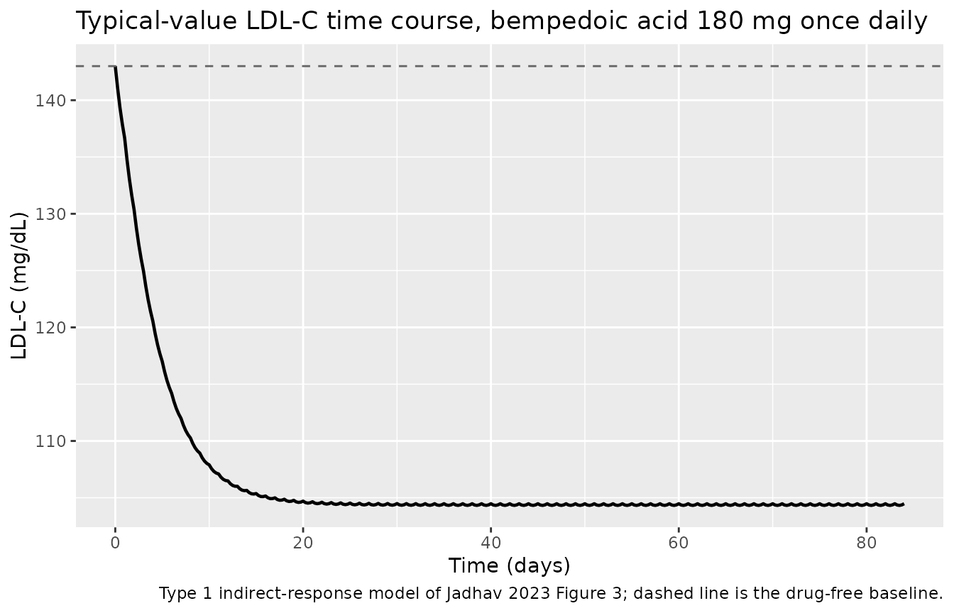
Jadhav 2023 reports a model-predicted LDL-C turnover of 85.8 h, and states that “the typical time required to achieve steady-state LDL-C concentrations following daily bempedoic acid dosing was approximately 3 weeks (99% of steady-state in 18 days)”.
pd_cov <- tibble::tibble(
  WT = 84.5, AGE = 62, CRCL = 89.3, SEXF = 0, RACE_BLACK = 0,
  DIS_HYPERLIP = 1, DIS_DIAB = 0, DIS_HEFH = 0,
  CONMED_EZE = 0, CONMED_SIMVASTATIN = 0, CONMED_ATORVASTATIN = 0,
  CONMED_STATIN_LI = 0, CONMED_STATIN_MI = 0, CONMED_STATIN_HI = 0,
  PRIOR_STATIN = 0, PRIOR_EZE = 0, FED = 0, SAMPLE_INTENSIVE = 0
)

pd_days <- 84
pd_events <- bind_rows(
  tidyr::crossing(pd_cov, time = seq(0, by = tau, length.out = pd_days)) |>
    mutate(amt = dose, evid = 1L, cmt = "depot"),
  tidyr::crossing(pd_cov, time = seq(0, pd_days * tau, by = 6)) |>
    mutate(amt = NA_real_, evid = 0L, cmt = "LDL")
) |>
  arrange(time, desc(evid))

sim_pd_typ <- rxode2::rxSolve(pdmod, events = pd_events, omega = NA) |>
  as.data.frame()
#> ℹ parameter labels from comments will be replaced by 'label()'

base_ldl <- sim_pd_typ$LDL[which.min(sim_pd_typ$time)]
ss_ldl   <- mean(sim_pd_typ$LDL[sim_pd_typ$time >= (pd_days - 1) * tau])
cfb      <- 100 * (ss_ldl - base_ldl) / base_ldl

# Day on which the response first reaches 99% of its eventual change.
t99 <- min(sim_pd_typ$time[
  (base_ldl - sim_pd_typ$LDL) >= 0.99 * (base_ldl - ss_ldl)
]) / 24

tibble::tibble(
  quantity = c("Baseline LDL-C (mg/dL)",
               "Week-12 LDL-C (mg/dL)",
               "Change from baseline (%)",
               "Days to 99% of the LDL-C change",
               "LDL-C turnover 1/kout (h)",
               "kout (1/day)"),
  model    = c(base_ldl, ss_ldl, cfb, t99, 85.8, 24 / 85.8),
  published = c(143, NA, -28, 18, 85.8, 0.3)
) |>
  dplyr::rename("Quantity" = quantity, "Model" = model, "Jadhav 2023" = published) |>
  knitr::kable(digits = 2,
caption = "Typical-value LDL-C response to bempedoic acid 180 mg once daily.")| Quantity | Model | Jadhav 2023 |
|---|---|---|
| Baseline LDL-C (mg/dL) | 143.00 | 143.0 |
| Week-12 LDL-C (mg/dL) | 104.40 | NA |
| Change from baseline (%) | -26.99 | -28.0 |
| Days to 99% of the LDL-C change | 17.50 | 18.0 |
| LDL-C turnover 1/kout (h) | 85.80 | 85.8 |
| kout (1/day) | 0.28 | 0.3 |
sim_pd_typ |>
  ggplot(aes(time / 24, LDL)) +
  geom_line(linewidth = 0.8) +
  geom_hline(yintercept = base_ldl, linetype = "dashed", colour = "grey40") +
  labs(
    x = "Time (days)",
    y = "LDL-C (mg/dL)",
    title = "Typical-value LDL-C time course, bempedoic acid 180 mg once daily",
    caption = "Type 1 indirect-response model of Jadhav 2023 Figure 3; dashed line is the drug-free baseline."
  )
Exposure-response relationship
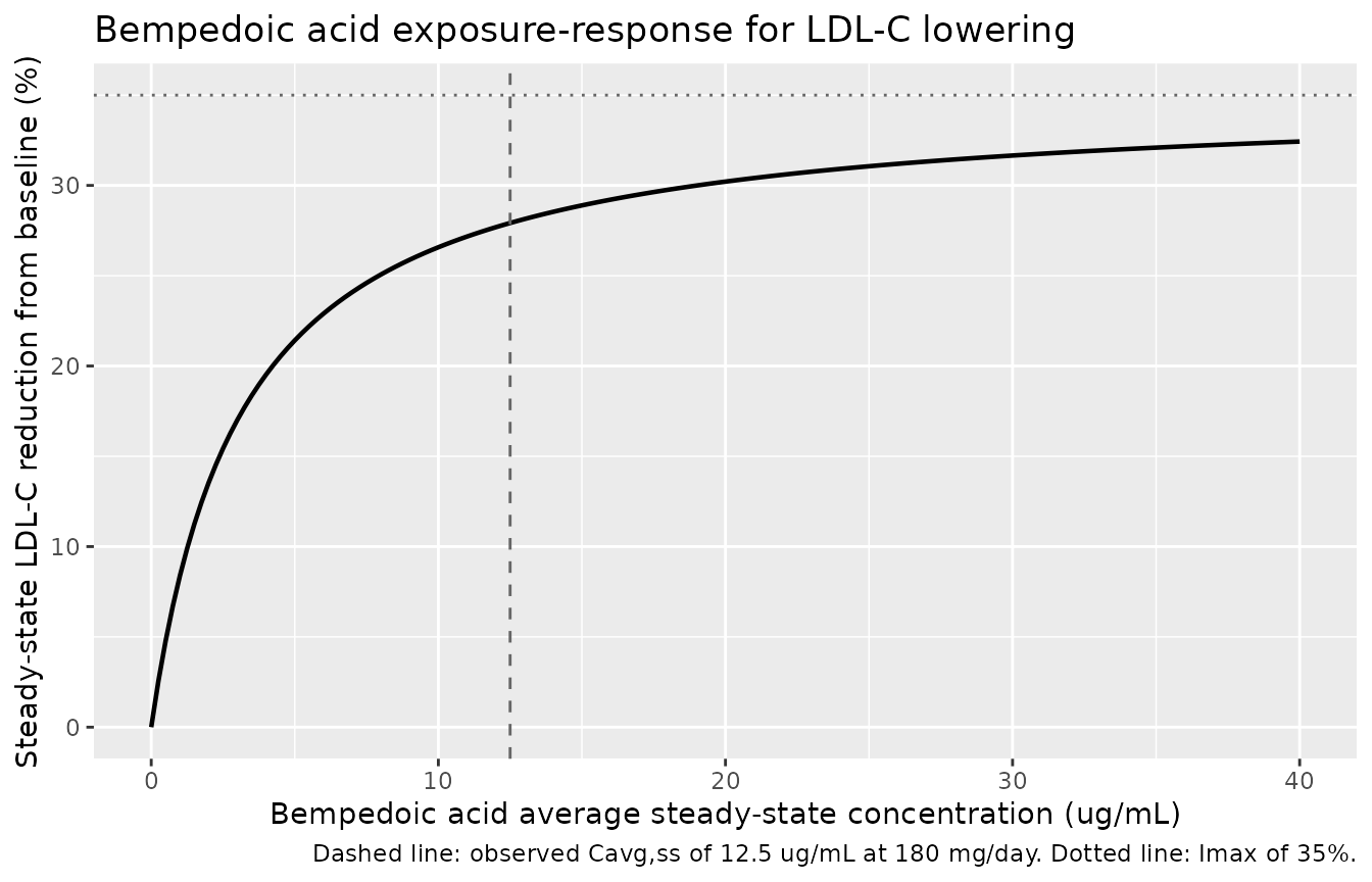
The Discussion states that at the observed average steady-state concentration of 12.5 ug/mL “a 28% reduction in LDL-C from baseline was predicted by the model, accounting for approximately 80% of the predicted Imax at 35% maximal inhibition”, and that 12.5 ug/mL is about 3.9-fold the estimated IC50 of 3.17 ug/mL.
imax <- 0.350
ic50 <- 3.17
cavg <- 12.5

er <- tibble::tibble(
  quantity = c("Cavg,ss / IC50 (fold)",
               "Fraction of Imax achieved at Cavg,ss (%)",
               "Predicted LDL-C reduction at Cavg,ss (%)"),
  model    = c(cavg / ic50,
               100 * cavg / (ic50 + cavg),
               100 * imax * cavg / (ic50 + cavg)),
  published = c(3.9, 80, 28)
)

er |>
  dplyr::rename("Quantity" = quantity, "Model" = model, "Jadhav 2023" = published) |>
  knitr::kable(digits = 1,
caption = "Exposure-response algebra at the published average steady-state concentration.")| Quantity | Model | Jadhav 2023 |
|---|---|---|
| Cavg,ss / IC50 (fold) | 3.9 | 3.9 |
| Fraction of Imax achieved at Cavg,ss (%) | 79.8 | 80.0 |
| Predicted LDL-C reduction at Cavg,ss (%) | 27.9 | 28.0 |
tibble::tibble(conc = seq(0, 40, by = 0.25)) |>
  mutate(reduction = 100 * imax * conc / (ic50 + conc)) |>
  ggplot(aes(conc, reduction)) +
  geom_line(linewidth = 0.8) +
  geom_vline(xintercept = cavg, linetype = "dashed", colour = "grey40") +
  geom_hline(yintercept = 100 * imax, linetype = "dotted", colour = "grey40") +
  labs(
    x = "Bempedoic acid average steady-state concentration (ug/mL)",
    y = "Steady-state LDL-C reduction from baseline (%)",
    title = "Bempedoic acid exposure-response for LDL-C lowering",
    caption = paste("Dashed line: observed Cavg,ss of 12.5 ug/mL at 180 mg/day.",
                    "Dotted line: Imax of 35%.")
  )
Covariate scenarios (Online Resource 5)
Online Resource 5 tabulates model-predicted steady-state LDL-C and LDL-C change from baseline for each covariate contrast. As with Figure 2, those published values are marginal means over resampled covariate vectors, so a typical-value prediction that flips one covariate at a time is expected to differ in magnitude while matching the direction and rank ordering. The table below reproduces the scenarios that the model can address with a single covariate flip.
scenarios <- tibble::tribble(
  ~scenario,                       ~override,
  "Reference (male, no LMT)",      list(),
  "Female",                        list(SEXF = 1),
  "Black race",                    list(RACE_BLACK = 1),
  "Body weight 60 kg",             list(WT = 60),
  "Body weight 110 kg",            list(WT = 110),
  "Type 2 diabetes",               list(DIS_DIAB = 1),
  "HeFH",                          list(DIS_HEFH = 1),
  "Concomitant ezetimibe",         list(CONMED_EZE = 1),
  "Low-intensity statin",          list(CONMED_STATIN_LI = 1),
  "Moderate-intensity statin",     list(CONMED_STATIN_MI = 1),
  "High-intensity statin",         list(CONMED_STATIN_HI = 1),
  "Prior statin therapy",          list(PRIOR_STATIN = 1),
  "Prior ezetimibe therapy",       list(PRIOR_EZE = 1)
)

run_scenario <- function(override) {
  cov <- pd_cov
  for (nm in names(override)) cov[[nm]] <- override[[nm]]
  ev <- bind_rows(
    tidyr::crossing(cov, time = seq(0, by = tau, length.out = pd_days)) |>
      mutate(amt = dose, evid = 1L, cmt = "depot"),
    tidyr::crossing(cov, time = c(0, seq((pd_days - 1) * tau, pd_days * tau, by = 6))) |>
      mutate(amt = NA_real_, evid = 0L, cmt = "LDL")
  ) |>
    arrange(time, desc(evid))
  s <- rxode2::rxSolve(pdmod, events = ev, omega = NA) |> as.data.frame()
  b  <- s$LDL[which.min(s$time)]
  ss <- mean(s$LDL[s$time >= (pd_days - 1) * tau])
  tibble::tibble(baseline = b, ldlc_ss = ss, cfb_pct = 100 * (ss - b) / b)
}

or5 <- scenarios |>
  mutate(res = lapply(override, run_scenario)) |>
  select(scenario, res) |>
  tidyr::unnest(res)

or5 |>
  dplyr::rename(
    "Scenario"                  = scenario,
    "Baseline LDL-C (mg/dL)"    = baseline,
    "Week-12 LDL-C (mg/dL)"     = ldlc_ss,
    "Change from baseline (%)"  = cfb_pct
  ) |>
  knitr::kable(digits = 1,
caption = "Typical-value LDL-C scenarios; compare directions and rank order with Online Resource 5 of Jadhav 2023.")| Scenario | Baseline LDL-C (mg/dL) | Week-12 LDL-C (mg/dL) | Change from baseline (%) |
|---|---|---|---|
| Reference (male, no LMT) | 143.0 | 104.4 | -27.0 |
| Female | 143.0 | 95.2 | -33.4 |
| Black race | 143.0 | 112.6 | -21.2 |
| Body weight 60 kg | 143.0 | 109.6 | -23.4 |
| Body weight 110 kg | 143.0 | 100.1 | -30.0 |
| Type 2 diabetes | 133.5 | 95.9 | -28.2 |
| HeFH | 152.6 | 111.4 | -27.0 |
| Concomitant ezetimibe | 143.0 | 96.0 | -32.8 |
| Low-intensity statin | 120.3 | 95.5 | -20.6 |
| Moderate-intensity statin | 104.7 | 85.0 | -18.8 |
| High-intensity statin | 101.1 | 85.4 | -15.5 |
| Prior statin therapy | 100.7 | 83.6 | -16.9 |
| Prior ezetimibe therapy | 134.5 | 98.2 | -27.0 |
The scenario table reproduces every direction reported in Online Resource 5: females and patients on concomitant ezetimibe achieve a larger fractional LDL-C reduction; Black race, prior statin therapy, and concomitant statins of any intensity reduce it, with the magnitude ordered low < moderate < high intensity; higher body weight increases the fractional reduction slightly; HeFH raises and type 2 diabetes lowers baseline LDL-C. It also reproduces the paper’s central clinical observation that although the percentage reduction shrinks with statin intensity, the absolute steady-state LDL-C achieved on moderate- and high-intensity statins is similar, because the baseline these patients start from is already lower.
Two rows show a percentage change identical to the reference: HeFH
and prior ezetimibe therapy. That is a structural consequence of the
model rather than a simulation artefact – both covariates act only on
baseline LDL-C, and because kin = kout * baseline, scaling
the baseline scales the whole indirect-response system proportionally
and leaves the fractional response untouched. Online Resource 5
reports small non-zero differences for these contrasts (HeFH -26.07% vs
-23.08%) because its marginal simulation lets the correlated
Imax covariates vary along with the baseline covariate; a
one-covariate-at-a-time prediction cannot and should not show that.
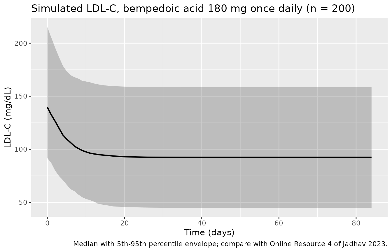
LDL-C variability
pd_subj <- subj |>
  select(id, SEXF, RACE_BLACK, DIS_HYPERLIP, DIS_DIAB, AGE, WT, CRCL,
         CONMED_EZE, CONMED_SIMVASTATIN, CONMED_ATORVASTATIN, FED) |>
  mutate(DIS_HEFH = 0,
         CONMED_STATIN_LI = 0, CONMED_STATIN_MI = 0, CONMED_STATIN_HI = 0,
         PRIOR_STATIN = 0, PRIOR_EZE = 0, SAMPLE_INTENSIVE = 0)

pd_pop_events <- bind_rows(
  tidyr::crossing(pd_subj, time = seq(0, by = tau, length.out = pd_days)) |>
    mutate(amt = dose, evid = 1L, cmt = "depot"),
  tidyr::crossing(pd_subj, time = seq(0, pd_days * tau, by = tau)) |>
    mutate(amt = NA_real_, evid = 0L, cmt = "LDL")
) |>
  arrange(id, time, desc(evid))

sim_pd_pop <- rxode2::rxSolve(pdmod, events = pd_pop_events) |> as.data.frame()

sim_pd_pop |>
  group_by(time) |>
  summarise(
    Q05 = quantile(LDL, 0.05),
    Q50 = quantile(LDL, 0.50),
    Q95 = quantile(LDL, 0.95),
    .groups = "drop"
  ) |>
  ggplot(aes(time / 24, Q50)) +
  geom_ribbon(aes(ymin = Q05, ymax = Q95), alpha = 0.25) +
  geom_line(linewidth = 0.8) +
  labs(
    x = "Time (days)",
    y = "LDL-C (mg/dL)",
    title = "Simulated LDL-C, bempedoic acid 180 mg once daily (n = 200)",
    caption = "Median with 5th-95th percentile envelope; compare with Online Resource 4 of Jadhav 2023."
  )
Assumptions and deviations
-
Covariate reference values are not printed in the source
paper. Jadhav 2023 Methods gives the covariate forms
theta_TV = theta_REF * (x / x_REF)^theta_x(continuous) andtheta_TV = theta_REF * (1 + theta_x * x)(categorical) but never statesx_REFfor body weight, age, or eGFR. The packaged models use the analysis-set medians reported in Table 1: 83.7 kg / 62.0 years / 89.3 mL/min for the PK layer (popPK analysis set) and 84.5 kg for the PDImaxweight exponent (bempedoic-acid-treated popPK/PD analysis set). Two lines of evidence support median normalisation over the 70 kg theory-based-allometry alternative: (i) the weight exponents were estimated (0.61 on CL/F, 0.94 on Vc/F) rather than fixed at 0.75 / 1, which is the pooled full-covariate-model idiom that normalises to the dataset median; and (ii) reconstructing the population mean Cavg,ss at 180 mg/day from the Table 2 coefficients and the Table 1 demographic mix gives 12.7 ug/mL with the median references versus 11.5 ug/mL with 70 kg / 90 mL/min, against the 12.5 ug/mL the paper reports. Only the absolute typical values of CL/F, Vc/F, and Imax depend on this choice; every published covariate ratio is invariant to it. A user who prefers the 70 kg convention can rescalelclby(83.7 / 70)^0.61andlvcby(83.7 / 70)^0.94. - Residual-error units typo in Table 3. The additive PD residual is printed as “3.94 g/dL”. Every LDL-C quantity in the paper is in mg/dL (baseline 143 mg/dL; observed median 113 mg/dL), so this is a units typographical error in the source and the value is packaged as 3.94 mg/dL. A 3.94 g/dL additive residual would be roughly 28-fold the mean response.
-
PD inter-individual variability distribution. Table
3 reports IIV magnitudes (43.1 %CV on Imax, 23.9 %CV on baseline LDL-C)
but the PD Methods does not restate the distributional form. The
log-normal assumption the paper declares for the popPK analysis
(“Interindividual variability was assumed to follow a log-normal
distribution”) is carried forward, so
omega^2 = log(CV^2 + 1). Note that a log-normalImaxis not bounded above by 1; at extreme positiveetalimaxcombined with severalImax-increasing covariates the inhibition fraction can exceed unity and the production term can go negative. This is a property of the published parameterisation, not of the encoding, and does not arise in the covariate ranges simulated here. -
No OMEGA off-diagonals are published. Both Table 2
and Table 3 report only diagonal %CV values, so the packaged models use
diagonal-only IIV. Any true correlation between
etalcl,etalvc, andetalka(or betweenetalimaxandetalrbase) is unrecoverable from the publication. -
Sequential PK/PD fitting is not reproduced. Jadhav
2023 fit the PD layer conditioned on individual post hoc PK parameters
(and, for the 33% of treated patients with no measurable concentrations,
on population-predicted concentrations).
Jadhav_2023_bempedoicAcid_ldlcinstead carries the full PK layer as ODEs so that it simulates end-to-end from a dose record. For simulation the two are equivalent; for re-estimation, a user reproducing the paper’s workflow should fix the PK parameters. - The metabolite ESP15228 is not modelled. The authors evaluated and then dropped it because it circulates at a roughly constant 20% of parent concentration, so parent drug is the surrogate for total active exposure (Methods, “Base structural model development”).
- Virtual-cohort covariate distributions are reconstructions. Table 1 reports marginal summaries only, so the cohort above samples each covariate independently from a distribution matched to the published median / mean / SD and truncated to the published range. The real correlations (notably between sex and body weight, and between age and eGFR) are not reproduced, which is precisely why the isolated model ratios in the Figure 2 table differ from the published marginal ratios.
- Published values compared here are marginal simulation summaries. Both Figure 2 and Online Resource 5 report the 50th (5th, 95th) percentiles of 100 parametric-bootstrap replicates over resampled covariate vectors. The comparisons in this article are typical-value or single-cohort predictions and are intended to confirm direction, rank order, and magnitude, not to reproduce those percentiles exactly. No parameter has been tuned to improve agreement.