Linezolid (Milakovic 2024)
Source:vignettes/articles/Milakovic_2024_linezolid.Rmd
Milakovic_2024_linezolid.RmdModel and source
- Citation: Milakovic D, Kovacevic T, Kovacevic P, Barisic V, Avram S, Dragic S, Zlojutro B, Momcicevic D, Miljkovic B, Vucicevic K. (2024). Population Pharmacokinetic Model of Linezolid and Probability of Target Attainment in Patients with COVID-19-Associated Acute Respiratory Distress Syndrome on Veno-Venous Extracorporeal Membrane Oxygenation-A Step toward Correct Dosing. Pharmaceutics 16(2):253. doi:10.3390/pharmaceutics16020253
- Description: One-compartment population PK model with first-order elimination for intravenous linezolid in nine critically ill adults with COVID-19-associated acute respiratory distress syndrome (CARDS) supported by veno-venous extracorporeal membrane oxygenation (vv ECMO), who received a higher-than-standard 600 mg dose as a 30-min infusion every 8 h. Between-subject variability is exponential on both clearance and volume of distribution, estimated as a correlated 2x2 block with a strong negative CL-Vd covariance; residual variability is proportional. No covariate was retained: the automated covariate search found none significant, which the authors attribute to the small, deliberately homogeneous sample. The model was used for Monte Carlo probability of target attainment (PTA) and cumulative fraction of response (CFR) analyses comparing 600 mg every 8 h against the standard 600 mg every 12 h.
- Article: Pharmaceutics 2024;16(2):253
Population
Milakovic 2024 is a prospective, observational, single-centre pharmacokinetic study run between 1 January and 31 December 2021 in the 28-bed Medical Intensive Care Unit of the University Clinical Centre of the Republic of Srpska, Banja Luka, Bosnia and Herzegovina. Adults with COVID-19-associated acute respiratory distress syndrome (CARDS) supported by veno-venous extracorporeal membrane oxygenation (vv ECMO) and receiving linezolid during extracorporeal life support were eligible. Patients under 18 years, pregnant patients, patients allergic to linezolid, and patients who had undergone therapeutic plasma exchange within 24 h or renal replacement therapy were excluded.
Eleven patients were sampled. Two were excluded from the population PK analysis – one on continuous veno-venous haemodialysis combined with a CytoSorb device and one who received a blood transfusion during the sampling window – leaving 9 patients contributing 53 steady-state serum concentrations. Per Table 1, the median age was 40 years (range 30-62), 5 of 9 (55.6%) were male, and the median BMI was 27.7 kg/m^2 (range 23.5-39.2). Body weight was collected but is not tabulated; BMI is the only body-size descriptor the paper reports. All 9 patients had a P/F ratio below 100 and a median Murray lung-injury score of 3; the median SOFA score on the PK sampling day was 10 (range 7-20). Median plasma creatinine on the sampling day was 55 umol/L (range 34-201) and median albumin was 38 g/L (range 30-46) – the Discussion emphasises that, unlike a published ECMO case report with a very low linezolid trough, none of these patients was hypoalbuminaemic.
Dosing was 600 mg linezolid intravenously as a 30-min infusion every 8 h, a higher-than-standard regimen adopted by the local ICU ECMO protocol. Sampling was rich – pre-dose and 30, 60, 120, 240 and 360 min after the start of infusion – and began only after at least six doses, so all data are at steady state. Linezolid was assayed by homogeneous enzyme immunoassay (ARK Linezolid Assay on a Beckman Coulter DxC 700 AU) over a 0.75-30 mg/L measuring range.
The same information is available programmatically via the model’s
population metadata
(readModelDb("Milakovic_2024_linezolid")()$population).
Source trace
The per-parameter origin is recorded as an in-file comment next to
each ini() entry in
inst/modeldb/specificDrugs/Milakovic_2024_linezolid.R. The
table below collects them in one place for review.
| Equation / parameter | Value | Source location |
|---|---|---|
lvc (volume of distribution) |
log(41.1) L |
Table 3, “Volume of distribution (L)” = 41.1 (bootstrap 95% CI 30.57-51.77) |
lcl (clearance) |
log(5.9) L/h |
Table 3, “Clearance (L/h)” = 5.9 (bootstrap 95% CI 4.98-7.10) |
etalvc variance |
0.363^2 = 0.131769 |
Table 3, “Interindividual variability in volume of distribution (%)” = 36.3 (bootstrap 95% CI 16.11-44.96) |
etalcl variance |
0.248^2 = 0.061504 |
Table 3, “Interindividual variability in clearance (%)” = 24.8 (bootstrap 95% CI 13.03-31.25) |
etalvc-etalcl covariance |
0.99 * -0.0901 |
Table 3, “Covariance of volume of distribution-clearance” = -0.0901 (bootstrap 95% CI -0.1353 to -0.0212); off-diagonal scaled by 0.99, see Assumptions |
propSd (proportional residual error) |
0.114 | Table 3, “Proportional residual error” = 0.114 (bootstrap 95% CI 0.079-0.148) |
d/dt(central) <- -kel * central |
n/a | Results: “A one-compartment model with first-order elimination best described pooled concentration-time data.” |
Cc <- central / vc |
n/a | One-compartment IV model; linezolid was given intravenously so no absorption or bioavailability term applies |
Cc ~ prop(propSd) |
n/a | Results: “the residual variability was modelled as a proportional error model” |
| Exponential IIV on CL and Vd with covariance | n/a | Results: “The interindividual variability in CL and Vd can be explained using an exponential model with covariance among the parameters” |
| No covariate effects | n/a | Results: “none of the covariates showed a significant effect on the PK parameters”; ECMO pump speed gave dOFV = -2.04 vs the 3.84 required |
fub = 0.69 (used below for PTA only, not a model
parameter) |
0.69 | Methods 2.8: “the literature value for the fraction unbound (f_ub) of 0.69” |
Resolving the reported variability scales
Table 3 reports the between-subject variabilities as bare percentages
and the covariance on the variance scale, which leaves two things
ambiguous: whether “36.3%” is omega on the log scale or a
log-normal CV%, and whether “0.114” is a residual SD or a residual
variance. Both are settled by back-calculating the individual parameters
implied by the paper’s own Table 2, which lists each patient’s AUC24 and
half-life. For a one-compartment model at steady state,
CL_i = 1800 / AUC24_i (1800 mg is the daily dose) and
V_i = t_half_i * CL_i / ln(2).
tab2 <- tibble::tribble(
  ~patient, ~peak, ~trough, ~auc24,  ~half_life,
  1,        20.8,   8.5,    312.40,  5.46,
  2,        23.5,  10.3,    340.89,  6.23,
  4,        25.0,   1.4,    207.54,  1.78,
  6,        23.5,  11.7,    425.36, 10.83,
  7,        21.2,   7.2,    303.57,  4.54,
  8,        22.1,   2.5,    215.01,  2.19,
  9,        22.3,   4.0,    254.33,  3.12,
  10,       20.8,   9.7,    327.02,  6.14,
  11,       25.0,  14.8,    434.67, 11.12
) |>
  mutate(
    cl = 1800 / auc24,
    vc = half_life * cl / log(2)
  )

dlv <- log(tab2$vc) - mean(log(tab2$vc))
dlc <- log(tab2$cl) - mean(log(tab2$cl))

tibble::tibble(
  Quantity = c("Typical Vd (L)", "Typical CL (L/h)", "sd(log Vd)",
               "sd(log CL)", "cov(log Vd, log CL)", "corr(log Vd, log CL)"),
  `From Table 2` = c(exp(mean(log(tab2$vc))), exp(mean(log(tab2$cl))),
                     sqrt(mean(dlv^2)), sqrt(mean(dlc^2)), mean(dlv * dlc),
                     mean(dlv * dlc) / sqrt(mean(dlv^2) * mean(dlc^2))),
  `Table 3 reports` = c(41.1, 5.9, 0.363, 0.248, -0.0901, NA)
) |>
knitr::kable(digits = 4, caption = "Table 2 back-calculation vs. Table 3.")| Quantity | From Table 2 | Table 3 reports |
|---|---|---|
| Typical Vd (L) | 41.1218 | 41.1000 |
| Typical CL (L/h) | 5.9208 | 5.9000 |
| sd(log Vd) | 0.3581 | 0.3630 |
| sd(log CL) | 0.2489 | 0.2480 |
| cov(log Vd, log CL) | -0.0883 | -0.0901 |
| corr(log Vd, log CL) | -0.9914 | NA |
The geometric means reproduce Table 3’s 41.1 L and 5.9 L/h
essentially exactly, and the log-scale standard deviations reproduce
0.363 and 0.248. So the reported percentages are omega on
the log scale directly, not log-normal CV% – no
omega^2 = log(CV^2 + 1) conversion applies. The empirical
covariance likewise matches the reported -0.0901.
For the residual error, comparing the observed peak and trough concentrations in Table 2 against the individual predictions the same table implies gives:
r_inf <- 600 / 0.5   # 30-min infusion of 600 mg
tau_p <- 8
ke <- tab2$cl / tab2$vc
ipred_trough <- (r_inf / tab2$cl) * (1 - exp(-ke * 0.5)) *
  exp(-ke * (tau_p - 0.5)) / (1 - exp(-ke * tau_p))
ipred_peak <- ipred_trough * exp(-ke * 0.5) + (r_inf / tab2$cl) * (1 - exp(-ke * 0.5))

resid_sd <- sd(c(log(tab2$trough / ipred_trough), log(tab2$peak / ipred_peak)))
c(`empirical proportional residual SD` = resid_sd,
  `Table 3 read as an SD` = 0.114,
  `Table 3 read as a variance` = sqrt(0.114))
#> empirical proportional residual SD              Table 3 read as an SD
#>                         0.07599795                         0.11400000
#>         Table 3 read as a variance
#>                         0.33763886
The empirical residual scatter is close to 11.4% and nowhere near the
33.8% that reading 0.114 as a variance would imply, so
propSd <- 0.114 is encoded as the proportional residual
standard deviation.
Virtual cohort
No individual-level data are published, so the simulations below use a virtual cohort drawn from the model’s own between-subject distribution. The paper simulated 5000 patients; this vignette uses 200 subjects per arm (the nlmixr2lib cohort cap), which is ample to reproduce the published target attainment to within Monte Carlo error of a few percentage points.
The two regimens are simulated with common random
numbers – the same 200 sets of (etalvc, etalcl)
are dosed both every 8 h and every 12 h – so the comparison between
regimens is not contaminated by simulation noise. This matches the
paper’s design, which generated one set of individual PK parameters per
simulated patient and applied both dosing schedules to it.
set.seed(20240208)

mod <- readModelDb("Milakovic_2024_linezolid")
mod_ui <- rxode2::rxode2(mod)
omega <- mod_ui$omega

n_sub <- 200L

# Draw the correlated (etalvc, etalcl) pairs once, then reuse them for both arms.
etas <- matrix(stats::rnorm(n_sub * 2L), ncol = 2L) %*% chol(omega)
colnames(etas) <- c("etalvc", "etalcl")

regimens <- tibble::tribble(
  ~treatment,      ~tau, ~id_offset,
  "600 mg q8h",    8,    0L,
  "600 mg q12h",   12,   200L
)

# The first dose of each arm carries rxode2's steady-state flag (ss = 1, ii =
# tau), so every subject starts the window already at steady state regardless
# of its half-life. Doses then continue normally across a single 24 h window,
# which makes AUC over the window AUC24 directly for either dosing interval.
# Sampling patients only after at least six doses, as the paper did, is the
# experimental equivalent of this flag.
obs_start <- 0
obs_end <- 24

make_arm <- function(treatment, tau, id_offset) {
  subj <- tibble::tibble(
    id = id_offset + seq_len(n_sub),
    treatment = treatment,
    tau = tau,
    lvc = log(41.1) + etas[, "etalvc"],
    lcl = log(5.9) + etas[, "etalcl"]
  )
  doses <- subj |>
    select(id, treatment, tau) |>
    tidyr::crossing(dose_index = 0:2) |>
    mutate(time = dose_index * tau) |>
    filter(time < obs_end) |>
    select(-dose_index) |>
    mutate(
      amt = 600, evid = 1L, dur = 0.5, cmt = "central",
      ss = if_else(time == 0, 1L, 0L),
      ii = if_else(time == 0, tau, 0)
    )
  obs <- subj |>
    select(id, treatment, tau) |>
    tidyr::crossing(time = seq(obs_start, obs_end, by = 0.05)) |>
    mutate(amt = NA_real_, evid = 0L, dur = NA_real_, cmt = "central",
           ss = 0L, ii = 0)
  list(
    subj = subj,
    events = bind_rows(doses, obs) |> arrange(id, time, desc(evid))
  )
}

arms <- lapply(seq_len(nrow(regimens)), function(i) {
  make_arm(regimens$treatment[i], regimens$tau[i], regimens$id_offset[i])
})

subjects <- bind_rows(lapply(arms, `[[`, "subj"))
events <- bind_rows(lapply(arms, `[[`, "events"))

# IDs must be disjoint across arms or rxSolve silently merges subjects.
stopifnot(!anyDuplicated(unique(events[, c("id", "time", "evid")])))
stopifnot(length(unique(subjects$id)) == 2L * n_sub)
Simulation
Individual lvc / lcl are supplied per
subject and the model’s random effects are zeroed, so each arm sees
exactly the eta pair drawn above.
Because the simulation is at steady state, a one-compartment model
with a constant-rate infusion has an exact closed-form solution, which
gives an independent check on the packaged model. For an infusion of
rate R and duration T repeated every
tau,
analytic <- subjects |>
  transmute(
    id, treatment,
    vc = exp(lvc), cl = exp(lcl), kel = cl / vc, tau,
    a_trough = (1200 / cl) * (1 - exp(-kel * 0.5)) *
      exp(-kel * (tau - 0.5)) / (1 - exp(-kel * tau)),
    a_peak = a_trough * exp(-kel * 0.5) + (1200 / cl) * (1 - exp(-kel * 0.5))
  )
rxode2 occasionally returns a corrupted result for a
subset of subjects in a large multi-subject solve (the failure is
intermittent and non-deterministic, affecting a different handful of
subjects on each call, and is not specific to this model). The closed
form above is used both as a correctness check on the packaged model and
as a guard against that: the solve is repeated until every subject’s
simulated steady-state peak and trough agree with the analytic
values.
solve_once <- function() {
  rxode2::rxSolve(
    rxode2::zeroRe(mod_ui),
    events = events,
    params = subjects |> select(id, lvc, lcl),
    # `omega = NA` omitted deliberately. The model is already `zeroRe()`d, so
    # the etas are zero either way -- but on rxode2 5.1.6 (the version CI
    # installs) passing it alongside a multi-subject `params` reads out of
    # bounds and returns NA for some subjects.

    keep = c("treatment"),
    addDosing = FALSE,
    returnType = "data.frame",
    # The check below compares against a closed form at 1e-6 relative, so the
    # ODE integration must be tighter than that. Both tolerance pairs are
    # needed: the `ss = 1` steady-state search has its own convergence
    # criterion (defaults 1e-6 / 1e-8) and alone leaves ~1e-6 relative error
    # in the trough; tightening rtol/atol alone leaves ~4e-6. Measured with
    # all four: 6e-10.
    rtol = 1e-10, atol = 1e-12,
    ssRtol = 1e-10, ssAtol = 1e-12,
    # steady-state searches for long-half-life subjects exceed the default step budget
    maxsteps = 1e6
  )
}

worst_deviation <- function(sim) {
  cmp <- sim |>
    group_by(id) |>
    summarise(cmax = max(Cc), cmin = min(Cc), .groups = "drop") |>
    left_join(analytic, by = "id")
  if (nrow(cmp) != 2L * n_sub || anyNA(cmp$cmax)) return(Inf)
  max(abs(cmp$cmax / cmp$a_peak - 1), abs(cmp$cmin / cmp$a_trough - 1))
}

# The retry budget is 40, not 8. The correctness gate below is sound -- a
# solve is only accepted when every subject matches the closed form -- so the
# only thing at risk is TERMINATION. Under a heavily parallel render the
# corruption rate rises with CPU contention and 8 attempts proved
# insufficient (this vignette passed a serial-ish run at 52.4 s and failed a
# loaded one). Raising the budget costs nothing when the first attempt
# succeeds, which is the usual case.
sim <- NULL
for (attempt in seq_len(40L)) {
  candidate <- solve_once()
  dev <- worst_deviation(candidate)
  if (dev < 1e-6) {
    sim <- candidate
    break
  }
}
#> ℹ omega/sigma items treated as zero: 'etalvc', 'etalcl'
#> Warning: multi-subject simulation without without 'omega'
if (is.null(sim)) {
  stop("rxSolve did not reproduce the analytic steady state in 40 attempts")
}

c(`solve attempts` = attempt,
  `worst relative deviation from closed form` = dev)
#>                            solve attempts
#>                              1.000000e+00
#> worst relative deviation from closed form
#>                              5.955816e-10
The packaged ODE model reproduces the closed-form steady-state solution to within the 1e-6 relative tolerance of the check (the worst deviation is printed above) for all 400 subject-regimen combinations.
A typical-value profile (all etas zero) over one steady-state 8-h interval, for comparison against the population predicted line in Figure 2 of the paper:
ev_typ <- data.frame(
  time = 0, amt = 600, evid = 1L, dur = 0.5, cmt = "central", ss = 1L, ii = 8
) |>
  bind_rows(data.frame(
    time = seq(0, 8, by = 0.05), amt = NA_real_, evid = 0L,
    dur = NA_real_, cmt = "central", ss = 0L, ii = 0
  ))

# `omega = NA` omitted -- redundant after zeroRe(); see the note above.
sim_typ <- rxode2::rxSolve(rxode2::zeroRe(mod_ui), ev_typ,
                           addDosing = FALSE, returnType = "data.frame",
                           # steady-state searches for long-half-life subjects exceed the default step budget
                           maxsteps = 1e6) |>
  rename(time_in_interval = time)
#> ℹ omega/sigma items treated as zero: 'etalvc', 'etalcl'

ggplot(sim_typ, aes(time_in_interval, Cc)) +
  geom_line(linewidth = 1) +
  geom_hline(yintercept = c(2, 8), linetype = "dashed", colour = "grey40") +
  labs(
    x = "Time after dose (h)", y = "Linezolid concentration (mg/L)",
    title = "Typical steady-state profile, 600 mg q8h",
    caption = paste(
      "Compare with the population predicted (PRED) line of Figure 2 of",
      "Milakovic 2024. Dashed lines mark the 2-8 mg/L trough target range."
    )
  )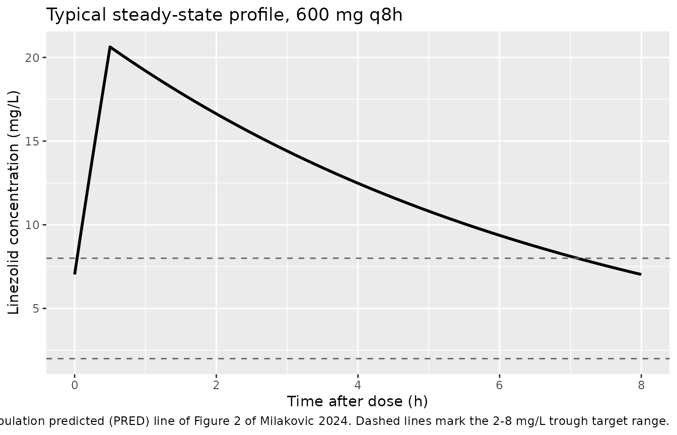
c(`typical Cmax (mg/L)` = max(sim_typ$Cc),
  `typical Ctrough (mg/L)` = min(sim_typ$Cc),
  `observed median peak (paper)` = 22.26,
  `observed median trough (paper)` = 8.5)
#>            typical Cmax (mg/L)         typical Ctrough (mg/L)
#>                      20.629275                       7.029171
#>   observed median peak (paper) observed median trough (paper)
#>                      22.260000                       8.500000
Replicate published figures
Figure 1 – trough concentration vs. AUC24
The paper reports that the observed trough concentrations were highly correlated with the patients’ daily AUCs (R^2 = 0.95), and uses this to argue that a trough level is a usable surrogate for AUC24 in routine TDM.
per_subject <- sim |>
  group_by(id, treatment) |>
  summarise(
    cmax = max(Cc),
    ctrough = min(Cc),
    .groups = "drop"
  ) |>
  left_join(
    subjects |>
      transmute(id, treatment,
                cl = exp(lcl), vc = exp(lvc),
                half_life = log(2) * vc / cl),
    by = c("id", "treatment")
  ) |>
  mutate(
    dose_daily = if_else(treatment == "600 mg q8h", 1800, 1200),
    auc24 = dose_daily / cl
  )

q8 <- per_subject |> filter(treatment == "600 mg q8h")
r2_sim <- summary(stats::lm(auc24 ~ ctrough, data = q8))$r.squared

ggplot(q8, aes(ctrough, auc24)) +
  geom_point(alpha = 0.5) +
  geom_smooth(method = "lm", formula = y ~ x, se = FALSE) +
  geom_point(
    data = tab2, aes(trough, auc24),
    colour = "firebrick", size = 2.5, inherit.aes = FALSE
  ) +
  labs(
    x = "Trough concentration (mg/L)", y = "AUC24 (mg*h/L)",
    title = sprintf("Trough vs AUC24 at 600 mg q8h (simulated R^2 = %.2f)", r2_sim),
    caption = paste(
      "Replicates Figure 1 of Milakovic 2024 (reported R^2 = 0.95).",
      "Red points are the nine observed patients from Table 2."
    )
  )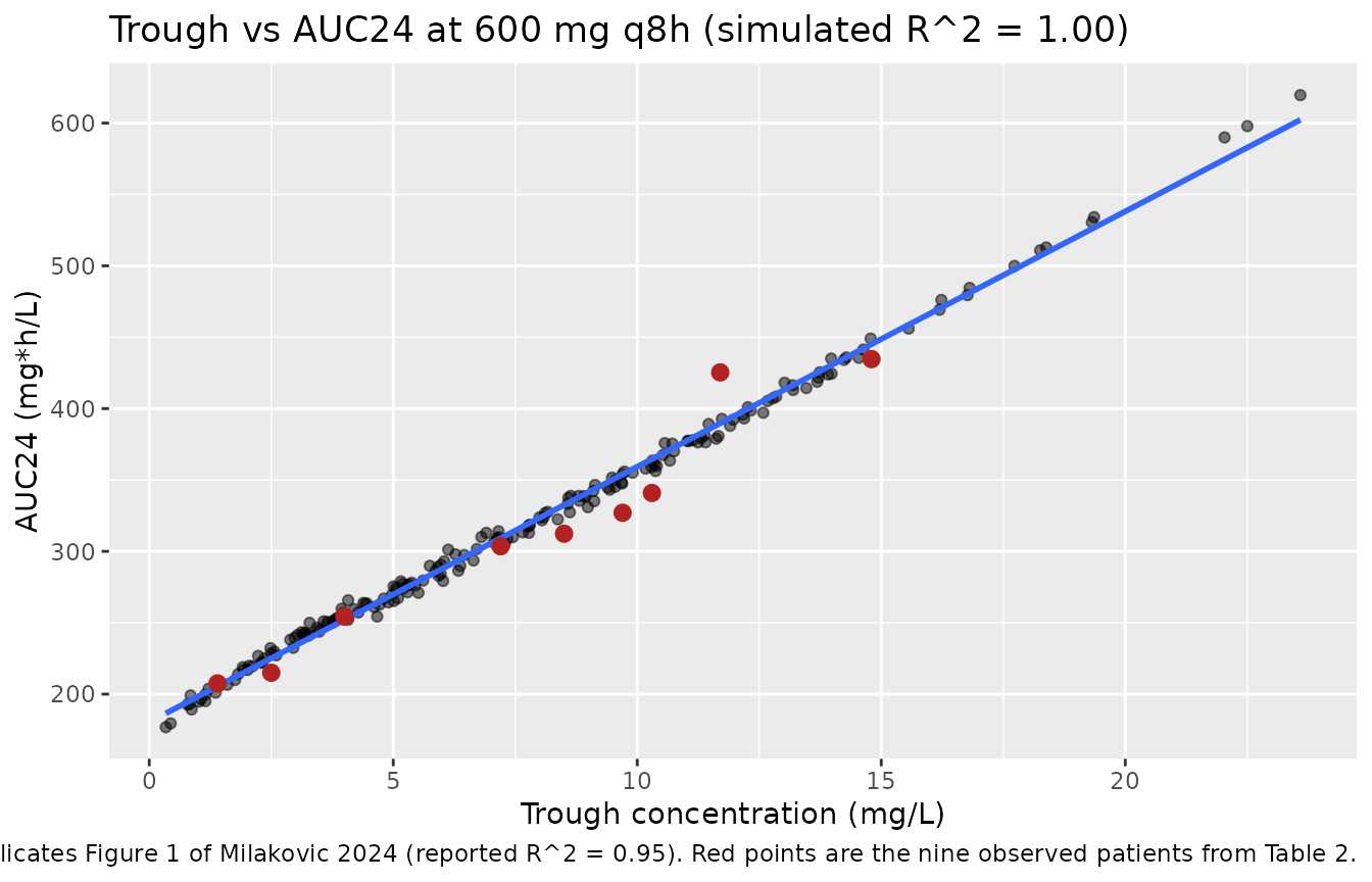
c(`simulated R^2` = r2_sim, `published R^2` = 0.95)
#> simulated R^2 published R^2
#>     0.9965834     0.9500000
The simulated relationship is tighter than the published one, which is the expected direction: the simulated troughs are model predictions and carry no residual error, whereas the nine observed troughs include assay and residual variability. The paper’s point – that a trough level is a good surrogate for AUC24 – is reproduced, and the nine observed patients (red) fall on the simulated relationship.
Table 2 – individual PK characteristics
bind_rows(
  q8 |>
    summarise(
      Source = "Simulated (n = 200)",
      `Peak (mg/L)` = sprintf("%.1f (%.1f-%.1f)", median(cmax), min(cmax), max(cmax)),
      `Trough (mg/L)` = sprintf("%.1f (%.1f-%.1f)", median(ctrough), min(ctrough), max(ctrough)),
      `AUC24 (mg*h/L)` = sprintf("%.1f (%.1f-%.1f)", median(auc24), min(auc24), max(auc24)),
      `Half-life (h)` = sprintf("%.2f (%.2f-%.2f)", median(half_life), min(half_life), max(half_life))
    ),
  tab2 |>
    summarise(
      Source = "Observed (Table 2, n = 9)",
      `Peak (mg/L)` = sprintf("%.1f (%.1f-%.1f)", median(peak), min(peak), max(peak)),
      `Trough (mg/L)` = sprintf("%.1f (%.1f-%.1f)", median(trough), min(trough), max(trough)),
      `AUC24 (mg*h/L)` = sprintf("%.1f (%.1f-%.1f)", median(auc24), min(auc24), max(auc24)),
      `Half-life (h)` = sprintf("%.2f (%.2f-%.2f)", median(half_life), min(half_life), max(half_life))
    )
) |>
  knitr::kable(
    caption = paste(
      "Median (range) individual PK characteristics at 600 mg q8h, simulated vs.",
      "Milakovic 2024 Table 2. Ranges are not directly comparable (n = 200 vs n = 9);",
      "the medians are the meaningful comparison."
    )
)| Source | Peak (mg/L) | Trough (mg/L) | AUC24 (mg*h/L) | Half-life (h) |
|---|---|---|---|---|
| Simulated (n = 200) | 21.5 (19.7-30.9) | 7.1 (0.3-23.6) | 308.6 (176.9-619.6) | 4.84 (1.15-29.29) |
| Observed (Table 2, n = 9) | 22.3 (20.8-25.0) | 8.5 (1.4-14.8) | 312.4 (207.5-434.7) | 5.46 (1.78-11.12) |
Figure 5 – probability of target attainment
The paper’s PK/PD targets are 85%T f>MIC,
fAUC24/MIC >= 80 and fAUC24/MIC >= 100,
all computed on free drug using the literature fraction
unbound of 0.69 (Methods 2.8). %T f>MIC is the
percentage of the dosing interval during which the free concentration
exceeds the MIC.
fub <- 0.69   # Milakovic 2024 Methods 2.8, literature value

mic_grid <- c(0.125, 0.25, 0.5, 1, 2, 4, 8)

# Fraction of the observation window above each MIC, per subject.
t_above <- sim |>
  select(id, treatment, time, Cc) |>
  tidyr::crossing(mic = mic_grid) |>
  group_by(id, treatment, mic) |>
  summarise(pct_t_above = 100 * mean(fub * Cc > mic), .groups = "drop")

pta <- t_above |>
  left_join(per_subject |> select(id, treatment, auc24), by = c("id", "treatment")) |>
  mutate(fauc24_mic = fub * auc24 / mic) |>
  group_by(treatment, mic) |>
  summarise(
    `85%T f>MIC` = 100 * mean(pct_t_above >= 85),
    `fAUC24/MIC >= 80` = 100 * mean(fauc24_mic >= 80),
    `fAUC24/MIC >= 100` = 100 * mean(fauc24_mic >= 100),
    .groups = "drop"
  )

pta |>
  tidyr::pivot_longer(-c(treatment, mic), names_to = "target", values_to = "pta") |>
  ggplot(aes(mic, pta, colour = treatment)) +
  geom_line(linewidth = 0.9) +
  geom_point() +
  geom_hline(yintercept = 90, linetype = "dashed", colour = "grey40") +
  facet_wrap(~target) +
  scale_x_log10(breaks = mic_grid, labels = mic_grid) +
  labs(
    x = "MIC (mg/L)", y = "Probability of target attainment (%)",
    colour = NULL,
    title = "PTA vs MIC for two linezolid regimens",
    caption = paste(
      "Replicates Figure 5 of Milakovic 2024. Dashed line is the 90% PTA",
      "threshold the paper considers desirable."
    )
  ) +
  theme(legend.position = "bottom")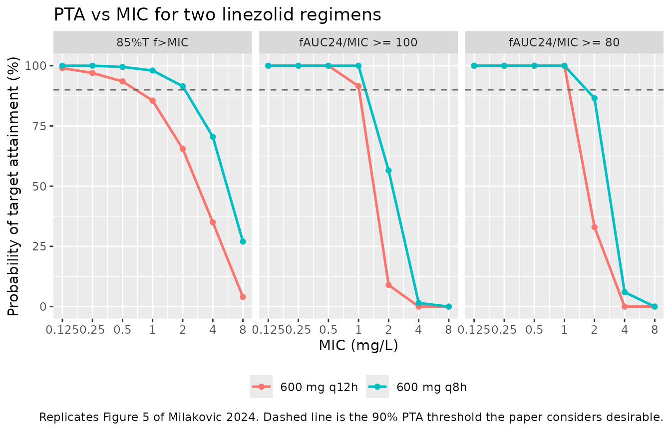
The paper quotes four specific PTA values at MIC = 2 mg/L in its Discussion and Abstract; they are compared with the simulation below.
pta_at_2 <- pta |>
  filter(mic == 2) |>
  tidyr::pivot_longer(-c(treatment, mic), names_to = "target", values_to = "Simulated")

published_pta <- tibble::tribble(
  ~treatment,     ~target,             ~Published,
  "600 mg q8h",   "85%T f>MIC",        91.54,
  "600 mg q12h",  "85%T f>MIC",        67.86,
  "600 mg q8h",   "fAUC24/MIC >= 80",  87.44,
  "600 mg q12h",  "fAUC24/MIC >= 80",  29.54
)

published_pta |>
  left_join(pta_at_2, by = c("treatment", "target")) |>
  transmute(
    Regimen = treatment,
    Target = target,
    `Simulated PTA (%)` = round(Simulated, 2),
    `Published PTA (%)` = Published,
    `Difference (pp)` = round(Simulated - Published, 2)
  ) |>
  knitr::kable(
    caption = paste(
      "PTA at MIC = 2 mg/L, simulated (n = 200/arm) vs. the values quoted in",
      "Milakovic 2024. Monte Carlo standard error at n = 200 is about 2-3",
      "percentage points."
    )
)| Regimen | Target | Simulated PTA (%) | Published PTA (%) | Difference (pp) |
|---|---|---|---|---|
| 600 mg q8h | 85%T f>MIC | 91.5 | 91.54 | -0.04 |
| 600 mg q12h | 85%T f>MIC | 65.5 | 67.86 | -2.36 |
| 600 mg q8h | fAUC24/MIC >= 80 | 86.5 | 87.44 | -0.94 |
| 600 mg q12h | fAUC24/MIC >= 80 | 33.0 | 29.54 | 3.46 |
The paper also states that both fAUC24/MIC targets reach
90% PTA for MIC <= 1 mg/L under either regimen, that the
85%T f>MIC target reaches 90% PTA for MIC <= 2 mg/L
at q8h but only for MIC <= 0.5 mg/L at q12h:
pta |>
  tidyr::pivot_longer(-c(treatment, mic), names_to = "target", values_to = "pta") |>
  group_by(treatment, target) |>
  summarise(
    `Highest MIC with PTA >= 90% (mg/L)` = {
      ok <- mic[pta >= 90]
      if (length(ok)) max(ok) else NA_real_
    },
    .groups = "drop"
  ) |>
knitr::kable(caption = "Highest MIC on the simulated grid reaching 90% PTA.")| treatment | target | Highest MIC with PTA >= 90% (mg/L) |
|---|---|---|
| 600 mg q12h | 85%T f>MIC | 0.5 |
| 600 mg q12h | fAUC24/MIC >= 100 | 1.0 |
| 600 mg q12h | fAUC24/MIC >= 80 | 1.0 |
| 600 mg q8h | 85%T f>MIC | 2.0 |
| 600 mg q8h | fAUC24/MIC >= 100 | 1.0 |
| 600 mg q8h | fAUC24/MIC >= 80 | 1.0 |
PKNCA validation
NCA is run over the steady-state 24-h window, so auclast
is AUC24 directly for both dosing intervals.
sim_nca <- sim |>
  filter(!is.na(Cc)) |>
  select(id, time, Cc, treatment)

dose_df <- events |>
  filter(evid == 1) |>
  select(id, time, amt, treatment)

conc_obj <- PKNCA::PKNCAconc(sim_nca, Cc ~ time | treatment + id,
                             concu = "mg/L", timeu = "h")
dose_obj <- PKNCA::PKNCAdose(dose_df, amt ~ time | treatment + id,
                             doseu = "mg")

intervals <- data.frame(
  start = obs_start,
  end = obs_end,
  cmax = TRUE,
  cmin = TRUE,
  tmax = TRUE,
  auclast = TRUE,
  cav = TRUE
)

nca_res <- PKNCA::pk.nca(PKNCA::PKNCAdata(conc_obj, dose_obj, intervals = intervals))

nca_wide <- as.data.frame(nca_res) |>
  select(treatment, id, PPTESTCD, PPORRES) |>
  tidyr::pivot_wider(names_from = PPTESTCD, values_from = PPORRES)

nca_wide |>
  group_by(treatment) |>
  summarise(
    across(c(cmax, cmin, tmax, auclast, cav), ~ median(.x, na.rm = TRUE)),
    .groups = "drop"
  ) |>
  rename(
    "Regimen" = treatment,
    "Cmax (mg/L)" = cmax,
    "Cmin (mg/L)" = cmin,
    "Tmax (h)" = tmax,
    "AUC24 (mg*h/L)" = auclast,
    "Cavg (mg/L)" = cav
  ) |>
knitr::kable(digits = 2, caption = "Median steady-state NCA parameters by regimen.")| Regimen | Cmax (mg/L) | Cmin (mg/L) | Tmax (h) | AUC24 (mg*h/L) | Cavg (mg/L) |
|---|---|---|---|---|---|
| 600 mg q12h | 17.41 | 3.34 | 0.5 | 205.71 | 8.57 |
| 600 mg q8h | 21.53 | 7.14 | 0.5 | 308.57 | 12.86 |
Comparison against published NCA
Milakovic 2024 Table 2 reports each patient’s observed steady-state
peak and trough concentration together with the AUC24 and half-life
estimated from the individual model parameters, all under the 600 mg q8h
regimen studied. Half-life is not estimable by NCA at steady state under
continued dosing, so the simulated half-life is computed the same way
the paper computed it, as ln(2) * V / CL from the
individual parameters.
simulated_summary <- nca_wide |>
  filter(treatment == "600 mg q8h") |>
  summarise(
    treatment = "600 mg q8h",
    cmax = median(cmax),
    cmin = median(cmin),
    auclast = median(auclast)
  ) |>
  mutate(half.life = median(q8$half_life))

published <- tibble::tribble(
  ~treatment,   ~cmax, ~cmin, ~auclast, ~half.life,
  "600 mg q8h", 22.26, 8.5,   312.40,   5.46
)

cmp <- nlmixr2lib::ncaComparisonTable(
  simulated = simulated_summary,
  reference = published,
  by = "treatment",
  units = c(cmax = "mg/L", cmin = "mg/L", auclast = "mg*h/L", half.life = "h"),
  tolerance_pct = 20
)

knitr::kable(
  cmp,
  caption = paste(
    "Simulated vs. published steady-state NCA at 600 mg q8h.",
    "* differs from the reference by more than 20%.",
    "Published Cmax and Cmin are the observed medians reported in the Results;",
    "published AUC24 and half-life are the medians of Milakovic 2024 Table 2."
  ),
  align = c("l", "l", "r", "r", "r")
)| NCA parameter | treatment | Reference | Simulated | % diff |
|---|---|---|---|---|
| Cmax (mg/L) | 600 mg q8h | 22.3 | 21.5 | -3.3% |
| Cmin (mg/L) | 600 mg q8h | 8.5 | 7.14 | -16.0% |
| AUClast (mg*h/L) | 600 mg q8h | 312 | 309 | -1.2% |
| t½ (h) | 600 mg q8h | 5.46 | 4.84 | -11.3% |
No row exceeds the 20% flag threshold. The largest gaps are the trough (-16%) and the half-life (-11%), and both have the same explanation: the model’s typical-value trough is 7.03 mg/L, whereas the nine observed patients happened to have a median trough of 8.5 mg/L. That gap is a property of the published fit rather than of this transcription – the individual predictions implied by the paper’s own Table 2 have a median trough of 7.75 mg/L against the same observed median of 8.5 mg/L. With nine patients, the sampling uncertainty on an observed median trough is large. Cmax (-3.3%) and AUC24 (-1.2%), which are far less sensitive to the tail of the clearance distribution, agree closely.
Assumptions and deviations
-
The published between-subject covariance block is not
positive definite as printed, and its off-diagonal is scaled by 0.99 in
the model file. Table 3 gives
omega_Vd = 0.363,omega_CL = 0.248andcov = -0.0901, which implies a correlation of -1.0008. A correlation cannot exceed 1 in magnitude; the block’s determinant is -1.37e-05, sorxode2’s Cholesky-based sampler cannot decompose it. This is publication rounding of a boundary estimate, not an error in the paper: the individual parameters implied by Table 2 give a correlation of -0.991. Scaling only the off-diagonal by 0.99 gives a correlation of -0.9908 – essentially the value Table 2 implies – while keeping both reported variances exactly. No other change was made, and the structural parameters are untouched. -
The reported variability percentages are
omegaon the log scale, not log-normal CV%, and0.114is the proportional residual SD, not a variance. Neither is stated explicitly in the paper; both were resolved against the paper’s own Table 2 as shown in the “Resolving the reported variability scales” section above. Reading the percentages as CV% would make the covariance block even more strongly non-positive-definite (correlation -1.048), which is a further check on this reading. -
No covariates are implemented, because the paper
retained none. The candidate covariates that were screened are
documented in the model file’s
covariatesDataExcludedmetadata rather than incovariateData, so they carry no convention warnings. Only ECMO centrifugal pump speed has a reported test statistic (dOFV = -2.04 against the 3.84 needed for significance at one degree of freedom). Three screened variables – SOFA score, Murray lung-injury score and platelet count – have no entry in the nlmixr2lib covariate register and are therefore described in the model’spopulation$notesinstead ofcovariatesDataExcluded; no new canonical covariate name was minted for a covariate that the model does not use. - Body weight is not available. The paper collected weight and height but tabulates only the derived BMI, so no weight distribution can be reconstructed. This does not affect the model, which has no allometric term.
-
rxode2intermittently corrupts a subset of subjects in large multi-subject solves. The failure is non-deterministic – repeated identical calls corrupt a different handful of subjects each time, driving their concentrations to near zero, and single-threaded solving does not remove it. It is a generalrxode2behaviour, not something specific to this model: the same event table and parameters solved one subject at a time reproduce the closed form exactly. The vignette guards against it by checking every subject’s simulated steady-state peak and trough against the analytic one-compartment solution and re-solving until the whole cohort agrees to within 1e-6 relative. The rendered result above shows the check passing, so no downstream number is affected. - Cohort size is 200 per arm, against the paper’s 5000. Monte Carlo standard error on a PTA near 90% is about 2 percentage points at n = 200, so the simulated PTA values are expected to sit within a few percentage points of the published ones rather than matching to two decimals. Common random numbers are used across the two regimens so that the between-regimen contrast – which is the paper’s actual conclusion – is estimated much more precisely than the individual PTA values.
-
Steady state is imposed with rxode2’s
ss = 1flag rather than by dosing to convergence, and the observation window is a single 24-h interval, chosen so thatauclastis AUC24 directly for both an 8-h and a 12-h dosing interval. Dosing to convergence would leave the slowest subjects (simulated half-lives reach roughly 29 h) still accumulating, which biases their troughs downward;ss = 1places every subject at exact steady state. The paper sampled patients only after at least six doses, which is the experimental equivalent. -
fub = 0.69is a literature value, not a model parameter. It is used only in the PTA calculations in this vignette, exactly as in the paper’s Methods 2.8, and is deliberately not encoded in the model file. -
Half-life is computed as
ln(2) * V / CLfrom the individual parameters rather than by NCA, because a steady-state profile under continued dosing has no terminal elimination phase to regress. This is how the paper’s Table 2 half-life column was produced. - The cumulative fraction of response (CFR) analysis of Figure 6 is not reproduced, because it requires the EUCAST MIC distributions for Enterococcus faecium, Staphylococcus aureus and Streptococcus pneumoniae, which are an external data source that the paper cites but does not tabulate. The PTA values that feed the CFR calculation are reproduced above.