Octreotide LAR (Kapralos 2021)
Source:vignettes/articles/Kapralos_2021_octreotide.Rmd
Kapralos_2021_octreotide.RmdModel and source
- Citation: Kapralos I, Dokoumetzidis A. Population Pharmacokinetic Modelling of the Complex Release Kinetics of Octreotide LAR: Defining Sub-Populations by Cluster Analysis. Pharmaceutics. 2021;13(10):1578. doi:10.3390/pharmaceutics13101578. Final-model estimates from Table 2; structural and variability equations from Equations 1-7 and Figure 1. The transit-compartment closed form follows Savic RM, Jonker DM, Kerbusch T, Karlsson MO. J Pharmacokinet Pharmacodyn. 2007;34(5):711-726.
- Description: One-compartment population PK model for octreotide after a single 30 mg intramuscular injection of the long-acting repeatable (LAR, Sandostatin LAR Depot) PLGA-microsphere formulation in healthy adult male volunteers. Release from the depot is a weighted sum of four processes: an initial burst dosed directly into a first-order absorption compartment, and three parallel delayed releases each described by the Savic (2007) closed-form transit density (Stirling approximation of n!) with its own mean transit time and transit count. The four fractions follow a multivariate logistic-normal distribution so they stay in (0, 1) and sum to one, the first mean transit time is logit-constrained below 300 h, and the second and third mean transit times are built as positive increments on the preceding one so the three delayed releases stay in sequential order. A binary subpopulation indicator from a pre-fit shape-respecting k-means clustering of the individual profiles (13% of subjects, early extended release) shifts the apparent clearance and the logits of the second and third release fractions. Single-dose model: the delayed-release inputs are driven by the most recent dose only.
- Article: https://doi.org/10.3390/pharmaceutics13101578
- Supplement (base-model Table S1 and goodness-of-fit figures): https://www.mdpi.com/article/10.3390/pharmaceutics13101578/s1
Octreotide LAR (Sandostatin LAR Depot) releases octreotide from PLGA
microspheres over about two months. Kapralos and Dokoumetzidis describe
the multi-peak release with an empirical input model: a small initial
burst plus three parallel delayed releases, each a Savic
transit-compartment density, feeding a first-order absorption
compartment and a one-compartment disposition model (Figure 1 of the
paper). Before the population fit, a shape-respecting k-means clustering
of the individual profiles split the subjects into a typical multi-phase
group (cluster 1) and an early extended-release group (cluster 2). The
cluster is carried as the binary covariate MIX_EARLY_REL (0
= cluster 1, 1 = cluster 2).
Population
118 healthy adult male Caucasian volunteers from the reference arm of a phase 1 single-dose bioequivalence study received one 30 mg deep intramuscular injection of Sandostatin LAR Depot under fasting conditions. Serum octreotide was sampled pre-dose and at 36 times from 0.5 h to 2088 h (3936 observations). Median (Q1-Q3) age was 28 (23-37) years, weight 75 (66-86) kg, height 175 (170-178) cm and BMI 24.75 (22.4-27.7) kg/m^2 (Table 1). The clustering assigned 103 subjects to cluster 1 and 15 (12.7%) to cluster 2 (Table 1).
The same information is available programmatically via
readModelDb("Kapralos_2021_octreotide")()$population.
Source trace
Every ini() value carries an in-file comment pointing to
its source in
inst/modeldb/specificDrugs/Kapralos_2021_octreotide.R. The
table collects them.
| Equation / parameter | Value | Source location |
|---|---|---|
lka |
log(0.27) 1/h | Table 2, ka |
lcl |
log(32.7) L/h | Table 2, CL |
lvc |
log(15.3) L | Table 2, V |
e_mix_early_rel_cl |
-8.61 L/h | Table 2, CL cluster effect; Equation 7 (additive) |
logitfburst |
-5.18 | Table 2, YF1 |
logitfdel1 |
-3.36 | Table 2, YF2 |
logitfdel2 |
-1.54 | Table 2, YF3 |
e_mix_early_rel_logitfdel1 |
3.06 | Table 2, YF2 cluster effect |
e_mix_early_rel_logitfdel2 |
-0.523 | Table 2, YF3 cluster effect |
mtt1max |
300 h (fixed) | Section 2.2.4, Equation 4 |
logitmtt1 |
-0.421 | Table 2, YMTT1 |
ldmtt2 |
log(181) h | Table 2, MTT2; Equation 3 increment |
ldmtt3 |
log(506) h | Table 2, MTT3; Equation 3 increment |
lnn1, lnn2, lnn3
|
log(3.42), log(17.9), log(5.08) | Table 2, N1-N3 |
| IIV variances | (CV/100)^2 | Table 2, IIV rows; CV definition in Section 2.2.4 |
propSd |
0.143 | Table 2, proportional residual error |
addSd |
28.4 pg/mL | Table 2, additive residual error |
Release fractions fburst-fdel3
|
n/a | Equation 5 and Figure 1 |
mtt1 logit constraint |
n/a | Equation 4 |
mtt2 = mtt1 + dmtt2,
mtt3 = mtt2 + dmtt3
|
n/a | Equation 3 |
ktr = (n + 1) / MTT |
n/a | Figure 1 |
| Transit density with Stirling n! | n/a | Equation 2 |
d/dt(depot) |
n/a | Equation 1; burst bolus from Figure 1 |
| Cluster effects additive on the typical value | n/a | Equation 7 |
Structural checks
Typical release fractions and transit times
mod <- readModelDb("Kapralos_2021_octreotide")
mod_typ <- rxode2::zeroRe(mod)
#> ℹ parameter labels from comments will be replaced by 'label()'

tgrid <- sort(unique(c(seq(0, 48, by = 0.1), seq(49, 6000, by = 1))))
make_typ <- function(mix, id) {
  dplyr::bind_rows(
    data.frame(id = id, time = 0, evid = 1, amt = 30, cmt = "depot"),
    data.frame(id = id, time = tgrid, evid = 0, amt = 0, cmt = "central")
  ) |>
    dplyr::mutate(MIX_EARLY_REL = mix)
}
ev_typ <- dplyr::bind_rows(make_typ(0, 1L), make_typ(1, 2L))
sim_typ <- rxode2::rxSolve(mod_typ, events = ev_typ, returnType = "data.frame") |>
  dplyr::mutate(cluster = ifelse(id == 1, "Cluster 1", "Cluster 2"))
#> ℹ omega/sigma items treated as zero: 'etalvc', 'etalcl', 'etalogitfburst', 'etalogitfdel1', 'etalogitfdel2', 'etalogitmtt1', 'etaldmtt2', 'etaldmtt3', 'etalnn1', 'etalnn2', 'etalnn3'
#> Warning: multi-subject simulation without without 'omega'

typ_par <- sim_typ |>
  dplyr::group_by(cluster) |>
  dplyr::slice(1) |>
  dplyr::ungroup() |>
  dplyr::select(cluster, cl, fburst, fdel1, fdel2, fdel3, mtt1, mtt2, mtt3, nn1, nn2, nn3)
knitr::kable(typ_par, digits = 4, caption = "Typical-subject parameters by cluster.")| cluster | cl | fburst | fdel1 | fdel2 | fdel3 | mtt1 | mtt2 | mtt3 | nn1 | nn2 | nn3 |
|---|---|---|---|---|---|---|---|---|---|---|---|
| Cluster 1 | 32.70 | 0.0045 | 0.0277 | 0.1709 | 0.7970 | 118.8832 | 299.8832 | 805.8832 | 3.42 | 17.9 | 5.08 |
| Cluster 2 | 24.09 | 0.0030 | 0.3954 | 0.0678 | 0.5338 | 118.8832 | 299.8832 | 805.8832 | 3.42 | 17.9 | 5.08 |
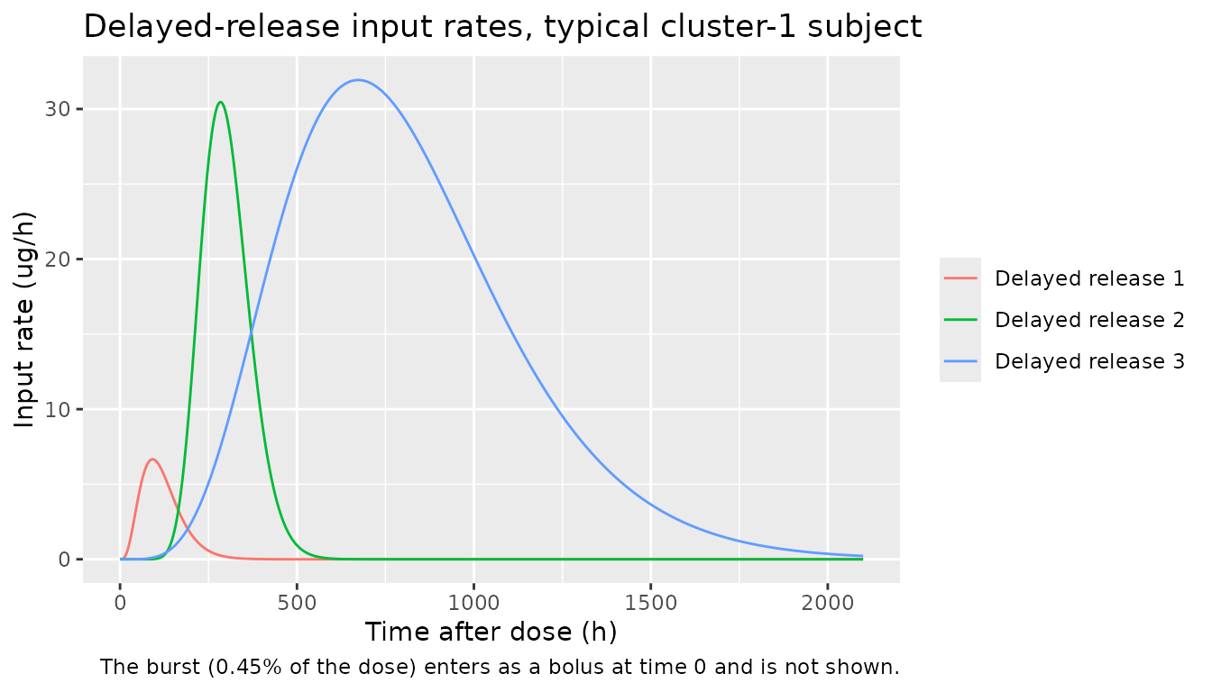
For cluster 1 the burst carries 0.45% of the dose, the first delayed
release 2.8%, the second 17.1% and the third 79.7%. The paper’s
statement that the initial burst accounts for less than 1/100 of the
total exposure (Discussion) matches fburst.
Sequential mean transit times (Equation 3)
Table 2 lists “MTT2” = 181 h and “MTT3” = 506 h. Equation 3 defines
MTT_j = MTT_(j-1) + theta_j * exp(eta_j), so the model
treats the two Table 2 values as the increments theta_2 and
theta_3, which gives MTT1 = 119 h, MTT2 = 300 h and MTT3 =
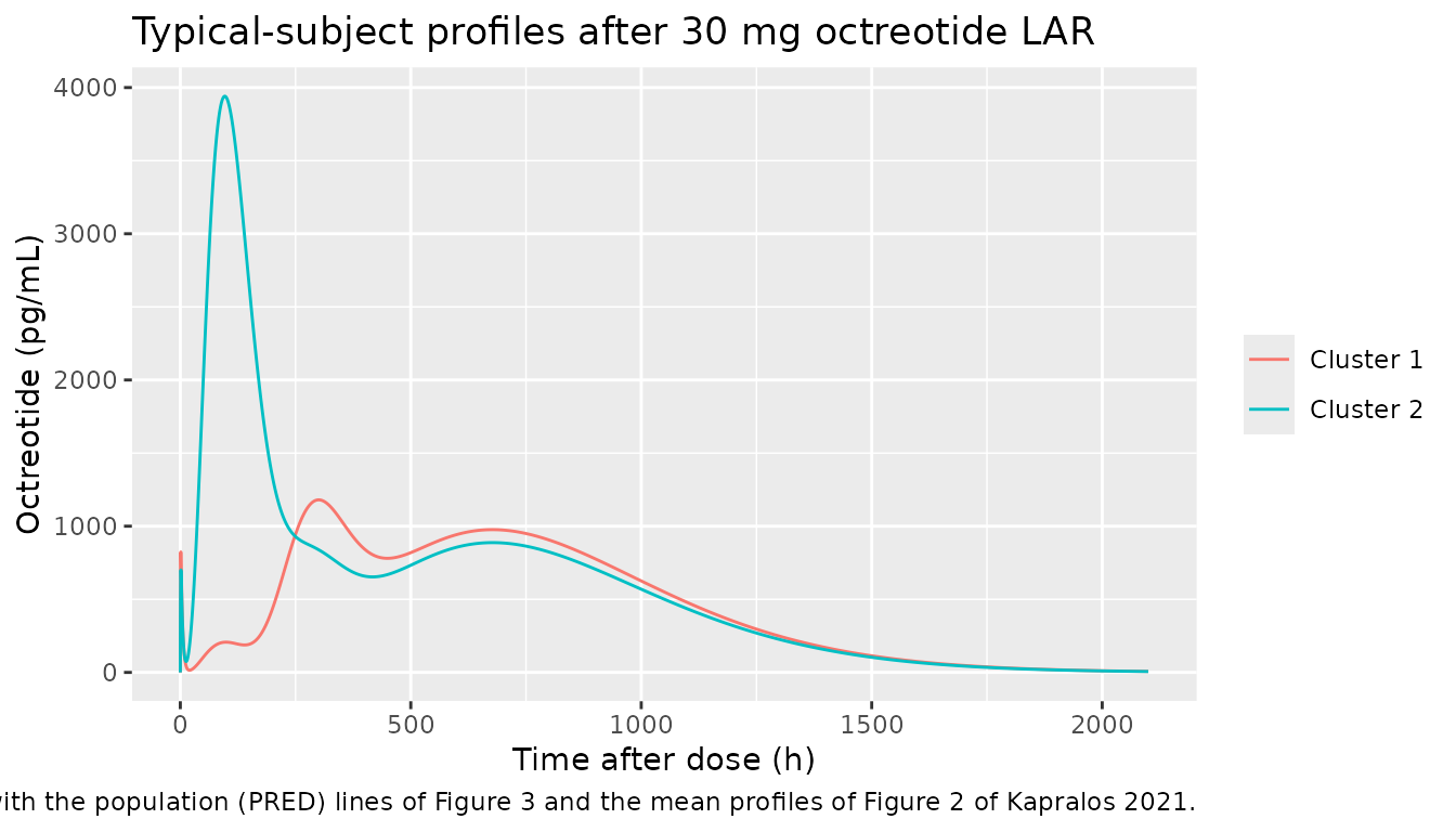
806 h. The published profiles support this reading. The mode of a Savic
input is at n / ktr = n * MTT / (n + 1), so the sharp
second delayed release (N2 = 17.9) peaks at about 284 h under the
increment reading. If 181 h were the absolute MTT2, it would peak at
about 171 h. Figure 2 (cluster-1 mean profile) and Figure 5 (VPC median)
both show the sharp second peak at about 300 h and a broad plateau
lasting past 1000 h. The broad plateau is what the third release
produces with a mean of 806 h, not 506 h.
typ1 <- sim_typ |> dplyr::filter(cluster == "Cluster 1", time > 48)
y <- typ1$Cc
local_max <- typ1$time[which(diff(sign(diff(y))) == -2) + 1]
local_max
#> [1]  99 300 677
# Deterministic typical-value gate: the second delayed peak must sit near the
# ~300 h peak of Figures 2 and 5, not at the ~171 h an absolute-MTT reading
# would put it.
stopifnot(any(local_max > 250 & local_max < 350))
Mass balance
The closed-form input uses Stirling’s approximation of
n! (Equation 2), so each delayed release delivers
Gamma(n + 1) / Stirling(n) of its fraction, slightly more
than one (about 1 + 1/(12 n)). For every subject the model
must therefore satisfy
CL * AUC(0-inf) = Dose * (fburst + sum_j f_j * Gamma(n_j + 1) / Stirling(n_j)).
Both sides use the same drawn parameters, so the check is tight. A
mutation control that drops the Stirling factor must fail, which shows
the gate can go red.
stir_factor <- function(n) exp(lgamma(n + 1) - (0.5 * log(2 * pi) + (n + 0.5) * log(n) - n))
mb <- sim_typ |>
  dplyr::group_by(cluster) |>
  dplyr::summarise(
    auc = sum(diff(time) * (head(Cc, -1) + tail(Cc, -1)) / 2) / 1e6, # mg*h/L
    cl = cl[1],
    expected = 30 * (fburst[1] + fdel1[1] * stir_factor(nn1[1]) +
      fdel2[1] * stir_factor(nn2[1]) + fdel3[1] * stir_factor(nn3[1])),
    naive = 30,
    .groups = "drop"
  ) |>
  dplyr::mutate(ratio = cl * auc / expected, ratio_naive = cl * auc / naive)
knitr::kable(mb, digits = 5)| cluster | auc | cl | expected | naive | ratio | ratio_naive |
|---|---|---|---|---|---|---|
| Cluster 1 | 0.93086 | 32.70 | 30.43928 | 30 | 1.00000 | 1.01464 |
| Cluster 2 | 1.26881 | 24.09 | 30.56577 | 30 | 0.99999 | 1.01885 |
stopifnot(
  all(abs(mb$ratio - 1) < 1e-3),
  # mutation control: ignoring the Stirling factor is detectably wrong
  all(abs(mb$ratio_naive - 1) > 5e-3)
)
The ratio of the typical AUCs is set by the cluster effect on CL, 32.7 / (32.7 - 8.61) = 1.357, times the small difference in the delivered amount (the two clusters split the dose differently across releases with different Stirling factors). The observed cluster AUC ratio is 1295.2 / 944.0 = 1.372 (Table 1).
typ_auc_ratio <- mb$auc[mb$cluster == "Cluster 2"] / mb$auc[mb$cluster == "Cluster 1"]
expected_ratio <- (32.7 / (32.7 - 8.61)) *
  mb$expected[mb$cluster == "Cluster 2"] / mb$expected[mb$cluster == "Cluster 1"]
c(simulated = typ_auc_ratio, expected = expected_ratio)
#> simulated  expected
#>  1.363045  1.363050
stopifnot(abs(typ_auc_ratio / expected_ratio - 1) < 1e-3)
Typical-value profiles
sim_typ |>
  dplyr::filter(time <= 2100) |>
  ggplot(aes(time, Cc, colour = cluster)) +
  geom_line() +
  labs(
    x = "Time after dose (h)", y = "Octreotide (pg/mL)", colour = NULL,
    title = "Typical-subject profiles after 30 mg octreotide LAR",
    caption = "Compare with the population (PRED) lines of Figure 3 and the mean profiles of Figure 2 of Kapralos 2021."
  )
The input rates of the four release processes for a typical cluster-1 subject show how the processes combine (Figure 1 of the paper).
sim_typ |>
  dplyr::filter(cluster == "Cluster 1", time <= 2100) |>
  dplyr::transmute(
    time,
    `Delayed release 1` = 30 * fdel1 * rin1,
    `Delayed release 2` = 30 * fdel2 * rin2,
    `Delayed release 3` = 30 * fdel3 * rin3
  ) |>
  tidyr::pivot_longer(-time, names_to = "process", values_to = "rate") |>
  ggplot(aes(time, rate * 1000, colour = process)) +
  geom_line() +
  labs(
    x = "Time after dose (h)", y = "Input rate (ug/h)", colour = NULL,
    title = "Delayed-release input rates, typical cluster-1 subject",
    caption = "The burst (0.45% of the dose) enters as a bolus at time 0 and is not shown."
  )
Virtual cohort and VPC
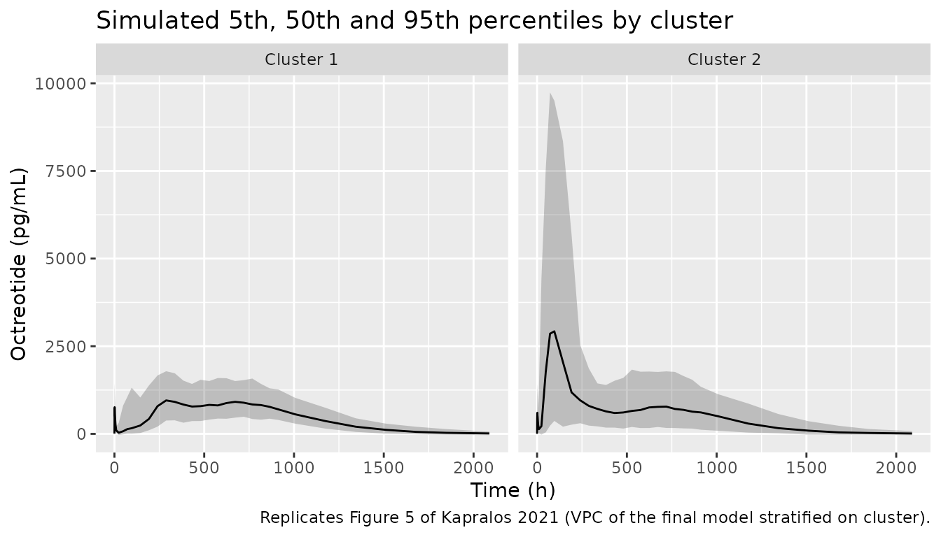
The paper’s VPC is stratified by cluster (Figure 5). The simulation uses 200 virtual subjects per cluster on the study’s sampling schedule. Body size and age were not retained as covariates, so the cohort needs no demographic columns.
rxode2::rxSetSeed(20211)
samp_times <- c(
  0, 0.5, 1, 1.5, 2, 3, 4, 6, 10, 24, 48, 72, 96, 144, 192, 240, 288, 336,
  384, 432, 480, 528, 576, 624, 672, 720, 768, 816, 864, 912, 1008, 1176,
  1344, 1512, 1680, 1848, 2088
)
make_cohort <- function(n, mix, id_offset = 0L) {
  ids <- id_offset + seq_len(n)
  dplyr::bind_rows(
    data.frame(id = ids, time = 0, evid = 1, amt = 30, cmt = "depot"),
    expand.grid(id = ids, time = samp_times) |>
      dplyr::mutate(evid = 0, amt = 0, cmt = "central")
  ) |>
    dplyr::mutate(
      MIX_EARLY_REL = mix,
      cluster = ifelse(mix == 1, "Cluster 2", "Cluster 1")
    ) |>
    dplyr::arrange(id, time, dplyr::desc(evid))
}
events <- dplyr::bind_rows(
  make_cohort(200, 0, id_offset = 0L),
  make_cohort(200, 1, id_offset = 200L)
)
stopifnot(!anyDuplicated(unique(events[, c("id", "time", "evid")])))
sim <- rxode2::rxSolve(mod, events = events, keep = "cluster", returnType = "data.frame")
#> ℹ parameter labels from comments will be replaced by 'label()'
sim |>
  dplyr::group_by(cluster, time) |>
  dplyr::summarise(
    Q05 = quantile(sim, 0.05, na.rm = TRUE),
    Q50 = quantile(sim, 0.50, na.rm = TRUE),
    Q95 = quantile(sim, 0.95, na.rm = TRUE),
    .groups = "drop"
  ) |>
  ggplot(aes(time, Q50)) +
  geom_ribbon(aes(ymin = Q05, ymax = Q95), alpha = 0.25) +
  geom_line() +
  facet_wrap(~cluster) +
  labs(
    x = "Time (h)", y = "Octreotide (pg/mL)",
    title = "Simulated 5th, 50th and 95th percentiles by cluster",
    caption = "Replicates Figure 5 of Kapralos 2021 (VPC of the final model stratified on cluster)."
  )
PKNCA validation
Table 1 reports arithmetic means of the observed AUC(0-t) and Cmax by
cluster. PKNCA runs on the simulated concentrations including residual
error (the sim column), because the observed values carry
assay noise. Values below the assay’s lower calibration limit (8.835
pg/mL) are set to zero before NCA. The paper’s Figure 6 partial AUCs
(0-24 h, 0-28 days and 28-56 days) are computed as well.
lloq <- 8.835
sim_nca <- sim |>
  dplyr::filter(!is.na(sim)) |>
  dplyr::transmute(id, time, cluster, conc = ifelse(sim < lloq, 0, sim))
sim_nca <- dplyr::bind_rows(
  sim_nca,
  sim_nca |> dplyr::distinct(id, cluster) |> dplyr::mutate(time = 0, conc = 0)
) |>
  dplyr::distinct(id, cluster, time, .keep_all = TRUE) |>
  dplyr::arrange(id, cluster, time)

conc_obj <- PKNCA::PKNCAconc(sim_nca, conc ~ time | cluster + id)
dose_df <- events |>
  dplyr::filter(evid == 1) |>
  dplyr::select(id, time, amt, cluster)
dose_obj <- PKNCA::PKNCAdose(dose_df, amt ~ time | cluster + id)

intervals <- data.frame(
  start = c(0, 0, 0, 672),
  end = c(2088, 24, 672, 1344),
  cmax = c(TRUE, FALSE, FALSE, FALSE),
  auclast = c(TRUE, FALSE, FALSE, FALSE),
  aucint.last = c(FALSE, TRUE, TRUE, TRUE)
)
nca_res <- PKNCA::pk.nca(PKNCA::PKNCAdata(conc_obj, dose_obj, intervals = intervals))
nca_long <- as.data.frame(nca_res$result)
Comparison against published NCA
# Table 1 reports arithmetic means; aggregate the simulated values the same way.
sim_means <- nca_long |>
  dplyr::filter(PPTESTCD %in% c("cmax", "auclast"), start == 0, end == 2088) |>
  dplyr::group_by(cluster, PPTESTCD) |>
  dplyr::summarise(PPORRES = mean(PPORRES, na.rm = TRUE), .groups = "drop")
# Whole cohort: weight the cluster means by the observed 103 / 15 split.
sim_means <- dplyr::bind_rows(
  sim_means,
  sim_means |>
    dplyr::group_by(PPTESTCD) |>
    dplyr::summarise(
      PPORRES = sum(PPORRES * ifelse(cluster == "Cluster 1", 103, 15)) / 118,
      .groups = "drop"
    ) |>
    dplyr::mutate(cluster = "All subjects")
)
published <- tibble::tribble(
  ~cluster,       ~cmax,  ~auclast,
  "Cluster 1",    1433.3, 944.0e3,
  "Cluster 2",    5034.8, 1295.2e3,
  "All subjects", 1891.1, 988.7e3
)
cmp <- nlmixr2lib::ncaComparisonTable(
  simulated = sim_means,
  reference = published,
  by = "cluster",
  units = c(cmax = "pg/mL", auclast = "pg*h/mL"),
  tolerance_pct = 20
)
knitr::kable(
  cmp,
  caption = "Simulated vs. published (Table 1) arithmetic-mean NCA. * differs from reference by >20%."
)| NCA parameter | cluster | Reference | Simulated | % diff |
|---|---|---|---|---|
| Cmax (pg/mL) | Cluster 1 | 1430 | 1480 | +3.3% |
| Cmax (pg/mL) | Cluster 2 | 5030 | 5210 | +3.5% |
| Cmax (pg/mL) | All subjects | 1890 | 1960 | +3.4% |
| AUClast (pg*h/mL) | Cluster 1 | 944000 | 949000 | +0.5% |
| AUClast (pg*h/mL) | Cluster 2 | 1300000 | 1310000 | +1.1% |
| AUClast (pg*h/mL) | All subjects | 989000 | 995000 | +0.6% |
The simulated means reproduce Table 1 closely in both clusters and in the whole cohort; no row is flagged.
chk <- sim_means |>
  dplyr::inner_join(
    tidyr::pivot_longer(published, -cluster, names_to = "PPTESTCD", values_to = "ref"),
    by = c("cluster", "PPTESTCD")
  ) |>
  dplyr::mutate(pct_diff = 100 * (PPORRES / ref - 1))
chk
#> # A tibble: 6 × 5
#>   cluster      PPTESTCD  PPORRES      ref pct_diff
#>   <chr>        <chr>       <dbl>    <dbl>    <dbl>
#> 1 Cluster 1    auclast   948833.  944000     0.512
#> 2 Cluster 1    cmax        1481.    1433.    3.32
#> 3 Cluster 2    auclast  1309365. 1295200     1.09
#> 4 Cluster 2    cmax        5212.    5035.    3.51
#> 5 All subjects auclast   994663.  988700     0.603
#> 6 All subjects cmax        1955.    1891.    3.38
# Rendered values were within 1.1% (AUC) and 3.5% (Cmax) of Table 1. The
# sampling standard error of a 200-subject mean is about 2% for AUC and 2.5-4%
# for Cmax (heavy upper tail from the YF2 IIV), so the envelopes below leave
# room for a different cohort draw while still catching a mis-scaled unit or
# a wrong cluster effect, either of which moves the means by tens of percent.
stopifnot(
  all(abs(chk$pct_diff[chk$PPTESTCD == "auclast"]) < 10),
  all(abs(chk$pct_diff[chk$PPTESTCD == "cmax"]) < 25)
)
The bioequivalence metrics of Figure 6 are summarised below as simulated 10th, 50th and 90th percentiles. The paper shows these only graphically, so they are not compared numerically.
nca_long |>
  dplyr::mutate(metric = dplyr::case_when(
    PPTESTCD == "cmax" ~ "Cmax (pg/mL)",
    PPTESTCD == "auclast" ~ "AUC(0-t) (pg*h/mL)",
    end == 24 ~ "AUC(0-24 h) (pg*h/mL)",
    end == 672 ~ "AUC(0-28 d) (pg*h/mL)",
    end == 1344 ~ "AUC(28-56 d) (pg*h/mL)"
  )) |>
  dplyr::filter(!is.na(metric), PPTESTCD %in% c("cmax", "auclast", "aucint.last")) |>
  dplyr::group_by(cluster, metric) |>
  dplyr::summarise(
    P10 = signif(quantile(PPORRES, 0.1, na.rm = TRUE), 3),
    P50 = signif(quantile(PPORRES, 0.5, na.rm = TRUE), 3),
    P90 = signif(quantile(PPORRES, 0.9, na.rm = TRUE), 3),
    .groups = "drop"
  ) |>
  dplyr::rename("Cluster" = cluster, "Metric" = metric) |>
knitr::kable(caption = "Simulated bioequivalence metrics (compare Figure 6 of Kapralos 2021).")| Cluster | Metric | P10 | P50 | P90 |
|---|---|---|---|---|
| Cluster 1 | AUC(0-24 h) (pg*h/mL) | 2910 | 4960 | 8150 |
| Cluster 1 | AUC(0-28 d) (pg*h/mL) | 287000 | 466000 | 729000 |
| Cluster 1 | AUC(0-t) (pg*h/mL) | 661000 | 916000 | 1290000 |
| Cluster 1 | AUC(28-56 d) (pg*h/mL) | 250000 | 390000 | 550000 |
| Cluster 1 | Cmax (pg/mL) | 879 | 1350 | 2040 |
| Cluster 2 | AUC(0-24 h) (pg*h/mL) | 3070 | 7230 | 30100 |
| Cluster 2 | AUC(0-28 d) (pg*h/mL) | 500000 | 850000 | 1300000 |
| Cluster 2 | AUC(0-t) (pg*h/mL) | 842000 | 1240000 | 1840000 |
| Cluster 2 | AUC(28-56 d) (pg*h/mL) | 106000 | 338000 | 664000 |
| Cluster 2 | Cmax (pg/mL) | 1540 | 4130 | 10100 |
Assumptions and deviations
-
MTT2 and MTT3 are increments. Table 2 labels the
two estimates “MTT2” and “MTT3”, but Equation 3 defines each later mean
transit time as the previous one plus
theta_j * exp(eta_j). The model uses the Table 2 values as those increments. The typical profile then puts the sharp second delayed peak at about 300 h and a plateau past 1000 h, as in Figures 2 and 5. Under the alternative reading the second peak would be at about 171 h and the third release would be exhausted by about 1000 h. See the structural checks above. -
IIV scale. Section 2.2.4 defines the reported IIV
as
CV(%) = sqrt(omega^2) * 100, so each variance is(CV/100)^2, including the logit-normal fraction and MTT1 parameters. - IIV covariances not reported. Section 3.2 states that the covariances between the fraction and the mean-transit-time etas were significant and kept. Neither Table 2 nor the supplementary Table S1 prints them, so the model carries a diagonal omega. Simulated between-subject spread of the release shape may therefore differ from the published VPC.
-
Residual error scale. Table 2 lists the
proportional (0.143) and additive (28.4 pg/mL) residual errors among the
fixed effects. The model treats them as standard deviations of a
combined error model. The paper does not say how the two components were
combined, so nlmixr2’s default
add() + prop()is used. -
Stirling approximation kept. Equation 2 replaces
n!in the Savic density with Stirling’s approximation. The model keeps this form because the parameters were estimated with it. As a result the total delivered amount slightly exceeds the dose (by about 1.5% for a typical subject); the mass-balance check above accounts for this exactly. -
No IIV on ka. Section 3.2 says IIV was estimated
for every parameter except ka. The base model in Table S1 shows ka IIV
as
0 FIXED. -
Single-dose model. The delayed-release inputs read
the most recent dose amount and time after dose (
podo()/tad()). With repeated monthly injections, a new dose would cut off the still-running release of the previous one (the release lasts about 2000 h). The paper studied a single dose only. Multiple-dose use would need superposition, which this model does not provide. -
Cluster covariate. The cluster assignment comes
from a pre-fit clustering of each subject’s observed profile. It cannot
be measured before dosing. For population simulation, draw
MIX_EARLY_REL ~ Bernoulli(15/118). - NCA inputs. The virtual cohort is 200 subjects per cluster. The whole-cohort NCA means weight the two clusters by the observed 103 / 15 split. Simulated concentrations below 8.835 pg/mL (the lowest calibration standard) were set to zero for NCA. The paper does not describe its below-limit handling.
- Errata. Crossref lists no correction or update to this article as of 2026-09-29.