Model and source
Khera et al. (2024) built a translational model chain for DYP688, an antibody-drug conjugate (ADC) against PMEL17 that carries two molecules of the Galpha-q/11 inhibitor FR900359. The payload inactivates (ring-opening) while it is still attached to the antibody, so a dose turns over time into ADC with two, one or no active payloads. The paper contributes six models to nlmixr2lib:
| Model | What it is |
|---|---|
Khera_2024_dyp688_mouse |
Mouse population PK (Table 1) |
Khera_2024_dyp688_fcrnmut_mouse |
Mouse PK of the fast-clearing FcRn-mut variant (Supplementary Table 2) |
Khera_2024_dyp688_mouse_tgi |
Mouse PK / tumour growth inhibition in 92.1 xenografts (Table 3) |
Khera_2024_dyp688_cyno |
Cynomolgus monkey population PK (Table 2) |
Khera_2024_dyp688_human |
Human PK projected allometrically from the monkey (Table 5) |
Khera_2024_dyp688_mouse_krogh_qsp |
Krogh cylinder QSP model of tumour delivery and Galpha-q/11 engagement (Supplementary Data, Supplementary Table 1) |
- Citation: Khera E, Dharmarajan L, Hainzl D, Engelhardt V, Vostiarova H, Davis J, Ebel N, Wuersch K, Romanet V, Sharaby S, Kearns JD. (2024). QSP modeling of a transiently inactivating antibody-drug conjugate highlights benefit of short antibody half life. J Pharmacokinet Pharmacodyn 52(1):7. doi:10.1007/s10928-024-09956-1.
- Article: https://doi.org/10.1007/s10928-024-09956-1 (open access, PMC11652588); the Supplementary Material holds the model equations, the Monolix model files and run summaries, and the Krogh cylinder parameters.
All PK models share one structure: a two-compartment model with
linear elimination for three ADC species distinguished by their number
of active payloads (dar2, dar1,
dar0), with each active payload inactivating at rate
kdec (the paper’s ki.a.) in both compartments. Because the
authors’ Monolix code splits every dose between the three species (1 -
fr into dar2, (1 - xfr) * fr into dar1, xfr *
fr into dar0), a dose is entered here as three records of
the same amount, one into each central compartment; f() in
the model does the split. Amounts are nmol of antibody.
# Nominal masses used only to convert mg/kg doses to nmol and nM to ug/mL.
# The paper does not state the ADC molecular weight or the animals' weights;
# see "Assumptions and deviations".
mw_adc <- 150000 # g/mol, nominal IgG-based ADC
mw_payload <- 1000 # g/mol, FR900359 (Supplementary Table 1, MW_P)
wt_mouse <- 0.020 # kg
wt_cyno <- 3 # kg (the paper's allometric-scaling weight)
wt_human <- 70 # kg (the paper's allometric-scaling weight)
mgkg_to_nmol <- function(mgkg, wt) mgkg * wt / mw_adc * 1e6

# One dose = the same amount into the three ADC-species central compartments.
dose_rows <- function(id, times, amt, dur = NULL) {
  d <- expand.grid(
    id = id, time = times,
    cmt = c("dar2_central", "dar1_central", "dar0_central"),
    stringsAsFactors = FALSE
  )
  d$amt <- amt
  d$evid <- 1L
  if (!is.null(dur)) d$dur <- dur
  d
}
# Observation rows for the multi-output PK models: none of the outputs is an
# ODE state, so the rows are keyed by dvid with no compartment.
obs_rows <- function(id, times) {
  expand.grid(id = id, time = times) |>
    mutate(evid = 0L, cmt = NA_character_, dvid = 1L)
}
Population
- Mouse PK: 16 female nude mice bearing subcutaneous 92.1-luc uveal melanoma xenografts, six IV treatment groups (3 and 6 mg/kg single doses; 1.5 mg/kg Q2W vs 3 mg/kg Q4W; 3 mg/kg Q2W vs 6 mg/kg Q4W). Total antibody and active / inactive ADC by ligand binding assays.
- Mouse PK / TGI: 24 xenograft mice in the four dose-fractionation groups plus saline vehicle (13 vehicle animals in the Gompertz growth fit).
- Cynomolgus monkey PK: 20 animals from a GLP toxicology study, 30 and 75 mg/kg slow IV bolus every two weeks for six doses; total antibody (serum LBA) and conjugated active / inactive payload (plasma papain-release LC-MS).
- Human projection: no human data in the fit; compared with interim Phase I PK (NCT05415072, 12 patients at 8 mg/kg Q2W).
The study details are in the Methods (“Preclinical in vivo study
design”, “Clinical study design”) and the Monolix run summaries in the
Supplementary Material. The same information is available
programmatically, e.g.
readModelDb("Khera_2024_dyp688_cyno")()$population.
Source trace
Every ini() value carries an in-file comment naming its
source. The table collects them. “Monolix output” is the run summary
printed in the Supplementary Material, which gives the estimates to one
more digit than Tables 1-3.
| Model / parameter | Value | Source |
|---|---|---|
| PK structure (all PK models) | – | Supplementary Data “Population PK-TGI model equations”; Monolix structure files (EQUATION blocks) |
Dose split f() (all PK models) |
1 - fr, (1 - xfr) fr, xfr fr | Monolix PK blocks, depot(target = ..., p = ...)
|
Mouse kel, k12, k21,
kdec, Vc
|
0.0161, 0.0355, 0.0356, 0.0125 1/h; 1.53 mL | Table 1; Monolix output |
Mouse fr, xfr, pinact,
pinact2
|
0.0274, 0.99 (fixed), 0.793, 0.161 | Table 1; Monolix output |
| Mouse IIV SD (kel, k12, k21, kdec, Vc) | 0.449, 0.15 (fixed), 0.26 (fixed), 0.0753, 0.03 (fixed) | Monolix output (Table 1 ‘IISD’) |
| Mouse residual (log scale) total Ab / active / inactive | 0.518 / 0.409 / 0.244 | Monolix output (see deviations) |
| Mouse residual percent payload a, b | 0.654, 0.209 | Table 1; Monolix output |
FcRn-mut Vc, kel, fr
(estimated) |
1.04 mL, 0.2709 1/h, 0.0082 | Supplementary Table 2 |
FcRn-mut k12, k21, kdec,
xfr, pinact, pinact2 (fixed) |
0.035, 0.036, 0.013, 0.99, 0.83, 0.18 | Supplementary Table 2 |
| FcRn-mut IIV SD (Vc, kel, k12, k21, kdec) | 0.04, 0.21, 0.15, 0.26, 0.075 | Supplementary Table 2 |
| TGI PK layer (fixed) | 0.016, 0.035, 0.036, 0.013 1/h; 1.53 mL; fr 0.027 | Monolix PK-TGI output |
TGI beta, TSmax (fixed) |
0.0059 1/h, 929 mm^3 | Table 3 (vehicle fit); Monolix PK-TGI output |
TGI kkill, dose-3 and dose-6 shifts |
0.000165 1/(nM h); 0.719; 1.18 | Table 3; Monolix PK-TGI output |
TGI tau
|
699 h | Table 3; Monolix PK-TGI output |
| TGI IIV SD kkill, tau | 0.897, 0.1 (fixed) | Table 3; Monolix PK-TGI output |
| TGI residual (log scale) | 0.734 | Table 3; Monolix PK-TGI output |
| TGI equations | – | Supplementary Data “Tumor growth inhibition model”; Monolix TGI structure file |
Cyno k12, k21, kdec,
Vc
|
0.0637, 0.0386, 0.0114 1/h; 0.0829 L | Table 2; Monolix output |
Cyno kel, fr, xfr
(fixed) |
0.0129 1/h, 0.01, 0.99 | Table 2 and footnote; Monolix output |
| Cyno IIV SD (k21, kdec, Vc) | 0.48 (fixed), 0.0624, 0.206 (fixed) | Table 2; Monolix output |
| Cyno proportional residual total Ab / active / inactive payload | 0.37 (fixed), 0.267, 0.725 | Table 2; Monolix output |
Human Vc, CL
|
1.93 L, 0.0251 L/h | Table 5, allometric equations (w = 1, 70 kg / 3 kg) |
Human k12, k21, inactivation t1/2,
fr
|
0.064, 0.039 1/h, 61 h, 1% | Table 5 |
| Krogh geometry, transport, binding, trafficking | see ini()
|
Supplementary Table 1 |
| Krogh equations and boundary conditions | – | Supplementary Data “Krogh cylinder model equations”, “Boundary conditions” |
| Tumorostatic concentration | TSC = beta log(TSmax / TS0) / kkill | Results, equation before Table 4 |
Mouse PK
mod_mouse <- readModelDb("Khera_2024_dyp688_mouse")

regimens <- tibble::tribble(
  ~regimen,           ~mgkg, ~tau, ~n_dose,
  "3 mg/kg SD",       3,     NA,   1,
  "6 mg/kg SD",       6,     NA,   1,
  "1.5 mg/kg Q2W",    1.5,   336,  3,
  "3 mg/kg Q4W",      3,     672,  2,
  "3 mg/kg Q2W",      3,     336,  3,
  "6 mg/kg Q4W",      6,     672,  2
) |>
  mutate(regimen = factor(regimen, levels = regimen))

n_per_group <- 40L
make_mouse_events <- function(i) {
  r <- regimens[i, ]
  ids <- (i - 1L) * n_per_group + seq_len(n_per_group)
  times <- if (is.na(r$tau)) 0 else seq(0, by = r$tau, length.out = r$n_dose)
  bind_rows(
    dose_rows(ids, times, mgkg_to_nmol(r$mgkg, wt_mouse)),
    obs_rows(ids, seq(0, 720, by = 6))
  ) |>
    mutate(regimen = r$regimen)
}
ev_mouse <- bind_rows(lapply(seq_len(nrow(regimens)), make_mouse_events)) |>
  arrange(id, time, desc(evid))

rxode2::rxSetSeed(2024)
sim_mouse <- rxode2::rxSolve(
  mod_mouse,
  events = ev_mouse, keep = "regimen", useLinCmt = FALSE,
  returnType = "data.frame"
)
#> ℹ parameter labels from comments will be replaced by 'label()'
# Replicates Figure 2A of Khera 2024 (median and 90% prediction interval of
# total antibody, active ADC and inactive ADC by treatment group).
sim_mouse |>
  select(id, time, regimen, `Total antibody` = Cc, `Active ADC` = Cc_active, `Inactive ADC` = Cc_inactive) |>
  pivot_longer(c(`Total antibody`, `Active ADC`, `Inactive ADC`), names_to = "analyte", values_to = "conc") |>
  filter(time > 0) |>
  group_by(regimen, analyte, time) |>
  summarise(
    q05 = quantile(conc, 0.05), q50 = median(conc), q95 = quantile(conc, 0.95),
    .groups = "drop"
  ) |>
  ggplot(aes(time, q50, colour = analyte, fill = analyte)) +
  geom_ribbon(aes(ymin = q05, ymax = q95), alpha = 0.15, colour = NA) +
  geom_line() +
  facet_wrap(~regimen, nrow = 2) +
  scale_y_log10(limits = c(1e-3, 2e3)) +
  scale_x_continuous(breaks = seq(0, 672, 168)) +
  labs(
    x = "Time (h)", y = "Concentration (nM)", colour = NULL, fill = NULL,
    caption = "Replicates Figure 2A of Khera 2024 (median, 90% prediction interval)."
  ) +
  theme(legend.position = "bottom")
#> Warning: Removed 146 rows containing missing values or values outside the scale range
#> (`geom_ribbon()`).
#> Warning: Removed 29 rows containing missing values or values outside the scale range
#> (`geom_line()`).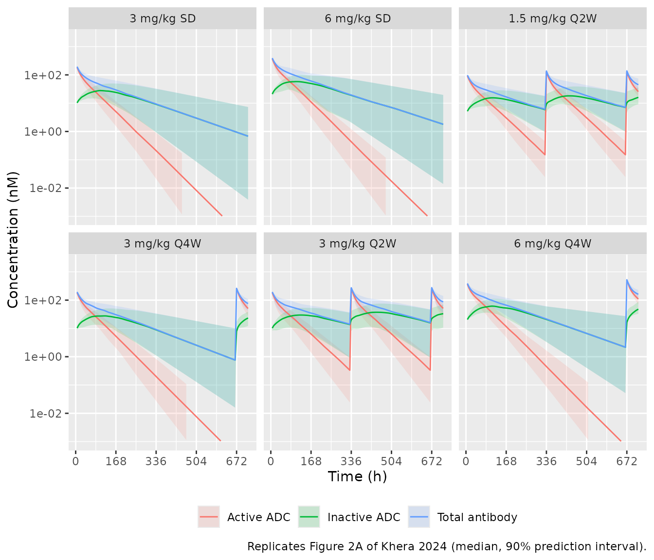
The active ADC falls much faster than total antibody, because the payload inactivation half-life (about two days) is shorter than the antibody half-life, and the inactive ADC rises to a broad peak, as in Figure 2A.
# Structural checks on the typical-value solution (deterministic, so the
# tolerances are numerical, not statistical).
typ_mouse <- rxode2::rxSolve(
  rxode2::zeroRe(mod_mouse),
  events = ev_mouse |> filter(id == 1), useLinCmt = FALSE, returnType = "data.frame"
)
#> ℹ parameter labels from comments will be replaced by 'label()'
#> ℹ omega/sigma items treated as zero: 'etalkel', 'etalk12', 'etalk21', 'etalkdec', 'etalvc'
total_p <- with(typ_mouse, 2 * (c_dar2 + c_dar1 + c_dar0))
stopifnot(
  # Total antibody is the sum of the three species.
  max(abs(typ_mouse$Cc - (typ_mouse$c_dar2 + typ_mouse$c_dar1 + typ_mouse$c_dar0))) < 1e-8,
  # Active payload percent stays within 0-100 and, straight after the first
  # dose, equals the vial composition: 100 * (1 - fr + (1 - xfr) * fr / 2).
  all(typ_mouse$active_payload_pct >= 0 & typ_mouse$active_payload_pct <= 100 + 1e-8),
  abs(typ_mouse$active_payload_pct[typ_mouse$time == 0][1] - 100 * (1 - 0.0274 + 0.01 * 0.0274 / 2)) < 1e-6
)
The in vivo inactivation half-life implied by kdec is
55.5 h in the mouse and 60.8 h in the monkey; the paper quotes “~52 h”
and “~61 h” (Results, after Table 2), with the in vitro mouse plasma
value at 39-42 h.
FcRn-mut variant
mod_fcrn <- readModelDb("Khera_2024_dyp688_fcrnmut_mouse")
ev_cmp <- bind_rows(
  dose_rows(1, 0, mgkg_to_nmol(12.5, wt_mouse)),
  obs_rows(1, c(0, seq(0.5, 24, by = 0.5), seq(25, 336, by = 1)))
)
cmp_fcrn <- bind_rows(
  rxode2::rxSolve(rxode2::zeroRe(mod_mouse), events = ev_cmp, useLinCmt = FALSE, returnType = "data.frame") |>
    mutate(molecule = "DYP688"),
  rxode2::rxSolve(rxode2::zeroRe(mod_fcrn), events = ev_cmp, useLinCmt = FALSE, returnType = "data.frame") |>
    mutate(molecule = "DYP688 FcRn-mut")
)
#> ℹ parameter labels from comments will be replaced by 'label()'
#> ℹ omega/sigma items treated as zero: 'etalkel', 'etalk12', 'etalk21', 'etalkdec', 'etalvc'
#> ℹ parameter labels from comments will be replaced by 'label()'
#> ℹ omega/sigma items treated as zero: 'etalvc', 'etalkel', 'etalk12', 'etalk21', 'etalkdec'

ggplot(cmp_fcrn |> filter(time > 0), aes(time, active_payload, colour = molecule)) +
  geom_line() +
  scale_y_log10() +
  labs(
    x = "Time (h)", y = "Conjugated active payload (nM)", colour = NULL,
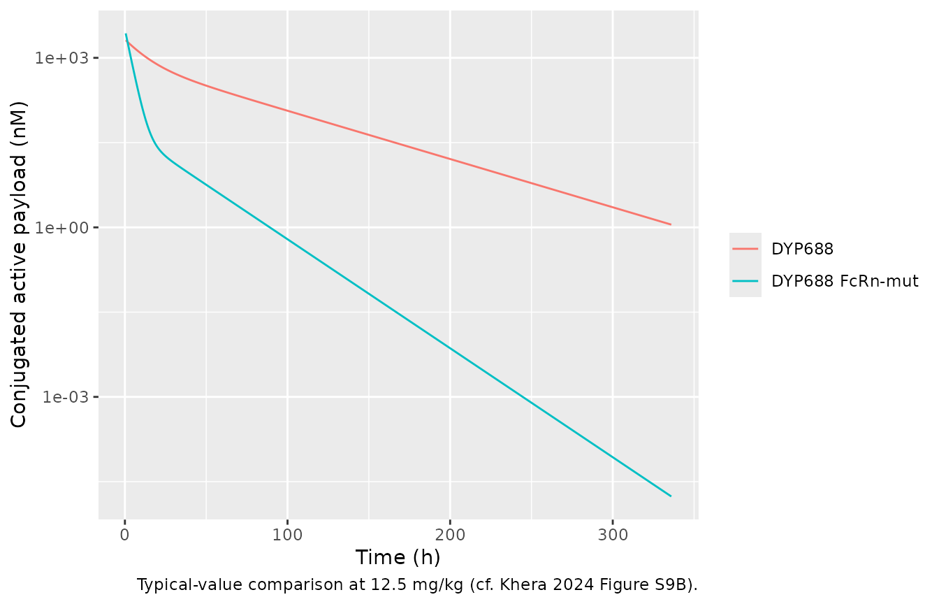
    caption = "Typical-value comparison at 12.5 mg/kg (cf. Khera 2024 Figure S9B)."
  )
cmp_fcrn |>
  group_by(molecule) |>
  summarise(
    `Cmax (nM)` = signif(max(active_payload), 3),
    `AUC0-336 (nM*h)` = signif(sum(diff(time) * (head(active_payload, -1) + tail(active_payload, -1)) / 2), 3),
    .groups = "drop"
  ) |>
knitr::kable(caption = "Same dose of the two molecules: FcRn-mut peaks somewhat higher (smaller Vc) but has about one fifth of the exposure.")| molecule | Cmax (nM) | AUC0-336 (nM*h) |
|---|---|---|
| DYP688 | 2120 | 56000 |
| DYP688 FcRn-mut | 3180 | 10900 |
Mouse PK / TGI
mod_tgi <- readModelDb("Khera_2024_dyp688_mouse_tgi")

tgi_regimens <- tibble::tribble(
  ~regimen,         ~mgkg, ~tau, ~n_dose,
  "Vehicle",        0,     NA,   0,
  "1.5 mg/kg Q2W",  1.5,   336,  4,
  "3 mg/kg Q4W",    3,     672,  2,
  "3 mg/kg Q2W",    3,     336,  4,
  "6 mg/kg Q4W",    6,     672,  2
) |>
  mutate(regimen = factor(regimen, levels = regimen))

make_tgi_events <- function(i) {
  r <- tgi_regimens[i, ]
  obs <- data.frame(id = i, time = seq(0, 1500, by = 12), evid = 0L, cmt = "tumor_size")
  ev <- if (r$n_dose > 0) {
    bind_rows(dose_rows(i, seq(0, by = r$tau, length.out = r$n_dose), mgkg_to_nmol(r$mgkg, wt_mouse)), obs)
  } else {
    obs
  }
  ev |>
    mutate(regimen = r$regimen, TUM_VOL = 250, DOSE_DYP688_MGKG = r$mgkg)
}
ev_tgi <- bind_rows(lapply(seq_len(nrow(tgi_regimens)), make_tgi_events)) |>
  arrange(id, time, desc(evid))

sim_tgi <- rxode2::rxSolve(
  rxode2::zeroRe(mod_tgi),
  events = ev_tgi, keep = "regimen", returnType = "data.frame"
)
#> ℹ parameter labels from comments will be replaced by 'label()'
#> ℹ omega/sigma items treated as zero: 'etalkel', 'etalk12', 'etalk21', 'etalkdec', 'etalvc', 'etalkkill', 'etaltau'
#> Warning: multi-subject simulation without without 'omega'

ggplot(sim_tgi, aes(time, tumor_size)) +
  geom_line() +
  facet_wrap(~regimen, nrow = 1) +
  labs(
    x = "Time (h)", y = "Tumour volume (mm^3)",
    caption = "Typical-value replication of Figure 3A of Khera 2024 (initial volume 250 mm^3)."
  )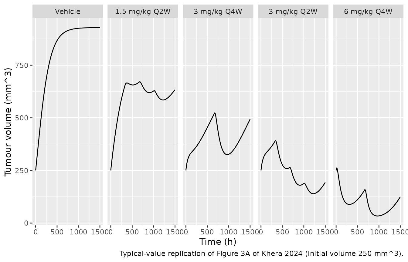
The typical tumour reaches the Gompertz plateau under vehicle, is held well below it by 1.5 mg/kg Q2W, rebounds between the two doses of 3 mg/kg Q4W, regresses slowly under 3 mg/kg Q2W and is held near its lowest volume by 6 mg/kg Q4W, the ordering of Figure 3A.
end_vol <- sim_tgi |>
  group_by(regimen) |>
  summarise(end = tumor_size[which.max(time)], .groups = "drop")
stopifnot(
  # Vehicle approaches TSmax = 929 mm^3 (Table 3).
  abs(end_vol$end[end_vol$regimen == "Vehicle"] - 929) / 929 < 0.01,
  # Dose fractionation ordering of Figure 3A: more frequent / higher dosing
  # gives smaller tumours.
  end_vol$end[end_vol$regimen == "3 mg/kg Q2W"] < end_vol$end[end_vol$regimen == "1.5 mg/kg Q2W"],
  end_vol$end[end_vol$regimen == "6 mg/kg Q4W"] < end_vol$end[end_vol$regimen == "3 mg/kg Q4W"]
)

cmax_tgi <- sim_tgi |>
  filter(regimen != "Vehicle") |>
  group_by(regimen) |>
  summarise(`Simulated Cmax of conjugated active payload (nM)` = round(max(active_payload)), .groups = "drop")
knitr::kable(cmax_tgi, caption = "Peak conjugated active payload by group; Figure 3B places the DYP688 groups at roughly 200-800 nM on its Cmax axis.")| regimen | Simulated Cmax of conjugated active payload (nM) |
|---|---|
| 1.5 mg/kg Q2W | 255 |
| 3 mg/kg Q4W | 509 |
| 3 mg/kg Q2W | 509 |
| 6 mg/kg Q4W | 1018 |
The kill rate constant has a categorical dose-level covariate. Table 4 lists the median of the individual estimates by dose; the typical values implied by the covariate model are close for 1.5 and 6 mg/kg, while the 3 mg/kg median of the individual estimates sits below the typical value.
kkill_pop <- 0.000165
tibble::tibble(
  Dose = c("1.5 mg/kg", "3 mg/kg", "6 mg/kg"),
  `Typical kkill (1/nM/h)` = signif(kkill_pop * exp(c(0, 0.719, 1.18)), 3),
  `Table 4 median kkill (1/nM/h)` = c(0.00016, 0.00026, 0.00058),
  `Table 4 TSC (nM)` = c(127, 34, 13.2)
) |>
knitr::kable(caption = "Kill rate constant by dose level (Khera 2024 Table 4).")| Dose | Typical kkill (1/nM/h) | Table 4 median kkill (1/nM/h) | Table 4 TSC (nM) |
|---|---|---|---|
| 1.5 mg/kg | 0.000165 | 0.00016 | 127.0 |
| 3 mg/kg | 0.000339 | 0.00026 | 34.0 |
| 6 mg/kg | 0.000537 | 0.00058 | 13.2 |
Cynomolgus monkey PK
mod_cyno <- readModelDb("Khera_2024_dyp688_cyno")
ev_cyno <- bind_rows(
  bind_rows(
    dose_rows(1, seq(0, by = 336, length.out = 6), mgkg_to_nmol(30, wt_cyno)),
    obs_rows(1, seq(0, 2016, by = 4))
  ) |> mutate(dose = "30 mg/kg"),
  bind_rows(
    dose_rows(2, seq(0, by = 336, length.out = 6), mgkg_to_nmol(75, wt_cyno)),
    obs_rows(2, seq(0, 2016, by = 4))
  ) |> mutate(dose = "75 mg/kg")
) |>
  arrange(id, time, desc(evid))
sim_cyno <- rxode2::rxSolve(
  rxode2::zeroRe(mod_cyno),
  events = ev_cyno, keep = "dose", useLinCmt = FALSE, returnType = "data.frame"
)
#> ℹ parameter labels from comments will be replaced by 'label()'
#> ℹ omega/sigma items treated as zero: 'etalk21', 'etalkdec', 'etalvc'
#> Warning: multi-subject simulation without without 'omega'
sim_cyno |>
  select(time, dose, `Total antibody` = Cc, `Conjugated active payload` = Cc_active_payload, `Conjugated inactive payload` = Cc_inactive_payload) |>
  pivot_longer(-c(time, dose), names_to = "analyte", values_to = "conc") |>
  filter(time > 0) |>
  ggplot(aes(time, conc, colour = analyte)) +
  geom_line() +
  facet_wrap(~dose) +
  scale_y_log10() +
  labs(
    x = "Time (h)", y = "Concentration (nM)", colour = NULL,
    caption = "Typical-value replication of Figure 2B of Khera 2024 (Q2W x 6)."
  ) +
  theme(legend.position = "bottom")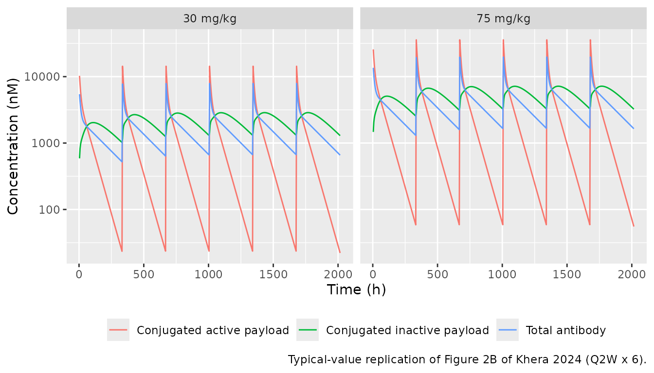
Human projection
Table 5 scales the monkey volume and clearance by body weight with exponent 1 (3 kg to 70 kg) and keeps the rate constants and inactivation half-life. The check below re-derives the human column from the monkey model.
cyno_vc <- 0.0829
cyno_cl <- 0.0129 * cyno_vc
tab5 <- tibble::tibble(
  Quantity = c("Cyno CL (L/h)", "Human Vc (L)", "Human CL (L/h)"),
  `Re-derived` = signif(c(cyno_cl, cyno_vc * 70 / 3, cyno_cl * 70 / 3), 3),
  `Table 5` = c(0.00108, 1.93, 0.0251)
)
knitr::kable(tab5, caption = "Allometric scaling re-derived from the monkey model vs Khera 2024 Table 5.")| Quantity | Re-derived | Table 5 |
|---|---|---|
| Cyno CL (L/h) | 0.00107 | 0.00108 |
| Human Vc (L) | 1.93000 | 1.93000 |
| Human CL (L/h) | 0.02500 | 0.02510 |
mod_human <- readModelDb("Khera_2024_dyp688_human")
n_human <- 100L
ev_human <- bind_rows(
  dose_rows(seq_len(n_human), 0, mgkg_to_nmol(8, wt_human), dur = 1.5),
  obs_rows(seq_len(n_human), c(0, 0.5, 1, 1.5, 2, 4, 6, 12, seq(24, 336, by = 12)))
) |>
  mutate(treatment = "8 mg/kg") |>
  arrange(id, time, desc(evid))
rxode2::rxSetSeed(2024)
sim_human <- rxode2::rxSolve(
  mod_human,
  events = ev_human, keep = "treatment", useLinCmt = FALSE,
  returnType = "data.frame"
) |>
  mutate(
    tab_ugml = Cc * mw_adc / 1e6,
    payload_ugml = Cc_active_payload * mw_payload / 1e6
  )
#> ℹ parameter labels from comments will be replaced by 'label()'
typ_human <- rxode2::rxSolve(
  rxode2::zeroRe(mod_human),
  events = ev_human |> filter(id == 1), useLinCmt = FALSE, returnType = "data.frame"
) |>
  mutate(tab_ugml = Cc * mw_adc / 1e6, payload_ugml = Cc_active_payload * mw_payload / 1e6)
#> ℹ parameter labels from comments will be replaced by 'label()'
#> ℹ omega/sigma items treated as zero: 'etalvc', 'etalk21', 'etalkdec'

# Arithmetic means of the interim clinical data at 8 mg/kg, cycle 1, read by
# the maintainers from Figure 6 of Khera 2024 (approximate).
fig6 <- tibble::tribble(
  ~time, ~analyte,                      ~obs,
  24,    "Total antibody",               115,
  72,    "Total antibody",               70,
  168,   "Total antibody",               45,
  336,   "Total antibody",               17,
  24,    "Conjugated active payload",    0.9,
  72,    "Conjugated active payload",    0.4,
  168,   "Conjugated active payload",    0.1,
  336,   "Conjugated active payload",    0.009
)
pred6 <- typ_human |>
  select(time, `Total antibody` = tab_ugml, `Conjugated active payload` = payload_ugml) |>
  pivot_longer(-time, names_to = "analyte", values_to = "pred")
cmp6 <- fig6 |>
  group_by(analyte) |>
  mutate(
    pred = approx(
      pred6$time[pred6$analyte == analyte[1]], pred6$pred[pred6$analyte == analyte[1]],
      xout = time
    )$y,
    ratio = pred / obs
  ) |>
  ungroup()

ggplot(pred6 |> filter(time > 0), aes(time, pred, colour = analyte)) +
  geom_line() +
  geom_point(data = fig6, aes(time, obs)) +
  scale_y_log10() +
  scale_x_continuous(breaks = c(0, 168, 336)) +
  labs(
    x = "Time (h)", y = "Concentration (ug/mL)", colour = NULL,
    caption = "Typical-value projection (lines) vs interim clinical means read from Figure 6 of Khera 2024 (points)."
  ) +
  theme(legend.position = "bottom")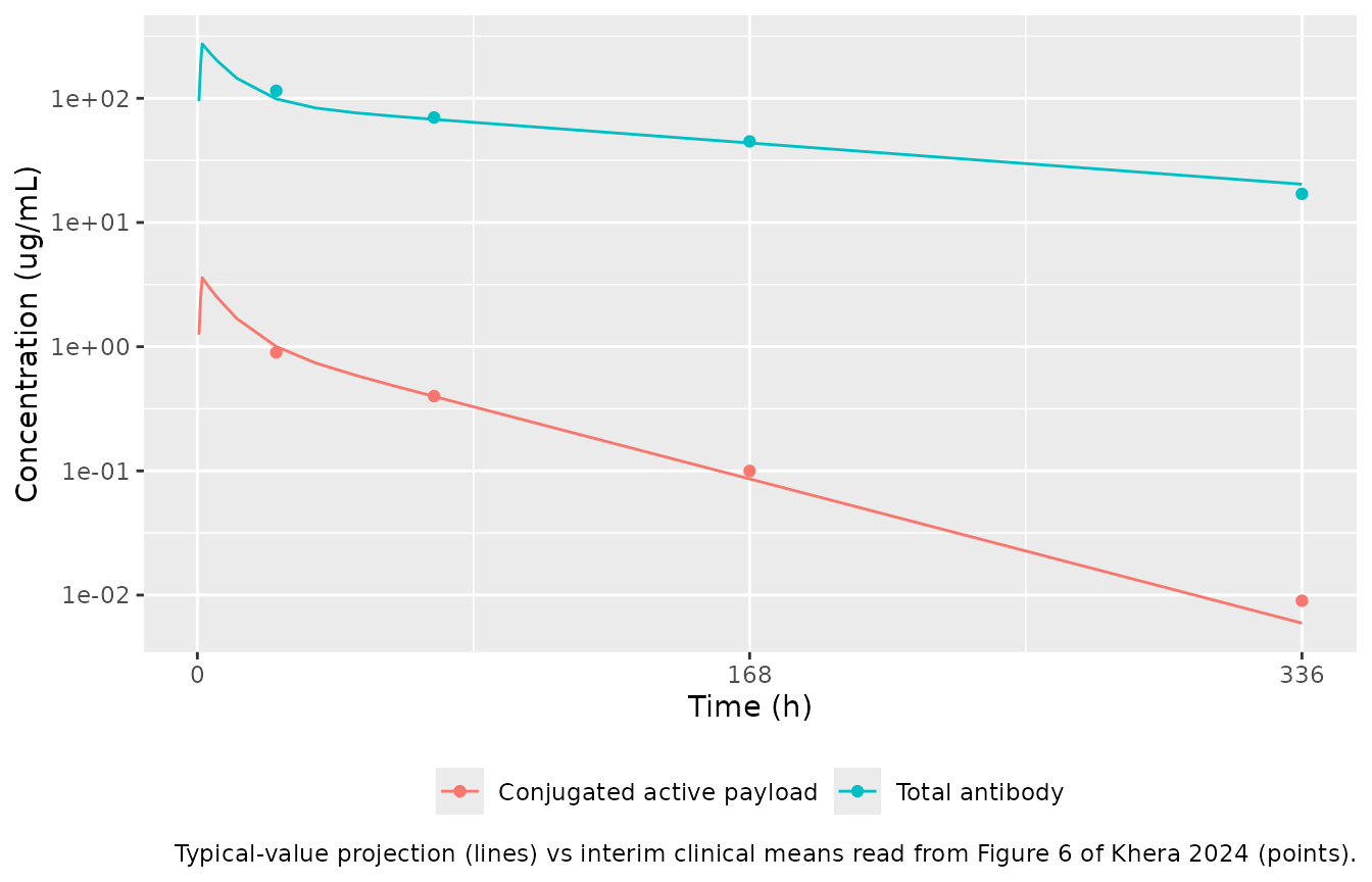
cmp6 |>
  mutate(pred = signif(pred, 3), ratio = round(ratio, 2)) |>
  select(analyte, time, `Figure 6 mean (ug/mL)` = obs, `Projection (ug/mL)` = pred, `Ratio` = ratio) |>
knitr::kable(caption = "Projection vs Figure 6 interim clinical data (8 mg/kg, cycle 1).")| analyte | time | Figure 6 mean (ug/mL) | Projection (ug/mL) | Ratio |
|---|---|---|---|---|
| Total antibody | 24 | 115.000 | 98.90000 | 0.86 |
| Total antibody | 72 | 70.000 | 67.70000 | 0.97 |
| Total antibody | 168 | 45.000 | 43.70000 | 0.97 |
| Total antibody | 336 | 17.000 | 20.30000 | 1.20 |
| Conjugated active payload | 24 | 0.900 | 1.00000 | 1.11 |
| Conjugated active payload | 72 | 0.400 | 0.39800 | 0.99 |
| Conjugated active payload | 168 | 0.100 | 0.08620 | 0.86 |
| Conjugated active payload | 336 | 0.009 | 0.00595 | 0.66 |
stopifnot(
  # Structural agreement with the interim clinical PK: a mis-scaled volume or
  # a wrong inactivation rate shifts these ratios by several-fold.
  abs(log(median(cmp6$ratio[cmp6$analyte == "Total antibody"]))) < log(1.5),
  abs(log(median(cmp6$ratio[cmp6$analyte == "Conjugated active payload"]))) < log(1.5)
)
PKNCA
The paper reports clinical NCA as having been run but does not tabulate it, so the table below gives the simulated NCA over the first 2-week dosing interval of the projection for reference (no published comparison is available).
nca_long <- sim_human |>
  select(id, time, treatment, `Total antibody` = Cc, `Conjugated active payload` = Cc_active_payload) |>
  pivot_longer(c(`Total antibody`, `Conjugated active payload`), names_to = "analyte", values_to = "Cc") |>
  filter(!is.na(Cc))
nca_long <- bind_rows(
  nca_long,
  nca_long |> distinct(id, treatment, analyte) |> mutate(time = 0, Cc = 0)
) |>
  distinct(id, treatment, analyte, time, .keep_all = TRUE) |>
  arrange(analyte, id, time)

conc_obj <- PKNCA::PKNCAconc(nca_long, Cc ~ time | treatment + analyte + id)
dose_df <- ev_human |>
  filter(evid == 1, cmt == "dar2_central") |>
  distinct(id, time, amt, treatment) |>
  tidyr::crossing(analyte = c("Total antibody", "Conjugated active payload"))
dose_obj <- PKNCA::PKNCAdose(dose_df, amt ~ time | treatment + analyte + id)
intervals <- data.frame(start = 0, end = 336, cmax = TRUE, tmax = TRUE, auclast = TRUE)
nca_res <- PKNCA::pk.nca(PKNCA::PKNCAdata(conc_obj, dose_obj, intervals = intervals))

as.data.frame(nca_res) |>
  filter(PPTESTCD %in% c("cmax", "tmax", "auclast")) |>
  group_by(analyte, PPTESTCD) |>
  summarise(median = signif(median(PPORRES), 3), .groups = "drop") |>
  pivot_wider(names_from = PPTESTCD, values_from = median) |>
  dplyr::rename(
    "Analyte" = analyte,
    "Cmax (nM)" = cmax,
    "Tmax (h)" = tmax,
    "AUC0-336 (nM*h)" = auclast
  ) |>
knitr::kable(caption = "Simulated NCA, 0-336 h after the first dose (median over 100 virtual 70 kg patients, 8 mg/kg over 1.5 h).")| Analyte | AUC0-336 (nM*h) | Cmax (nM) | Tmax (h) |
|---|---|---|---|
| Conjugated active payload | 99600 | 3600 | 1.5 |
| Total antibody | 118000 | 1830 | 1.5 |
Krogh cylinder QSP model
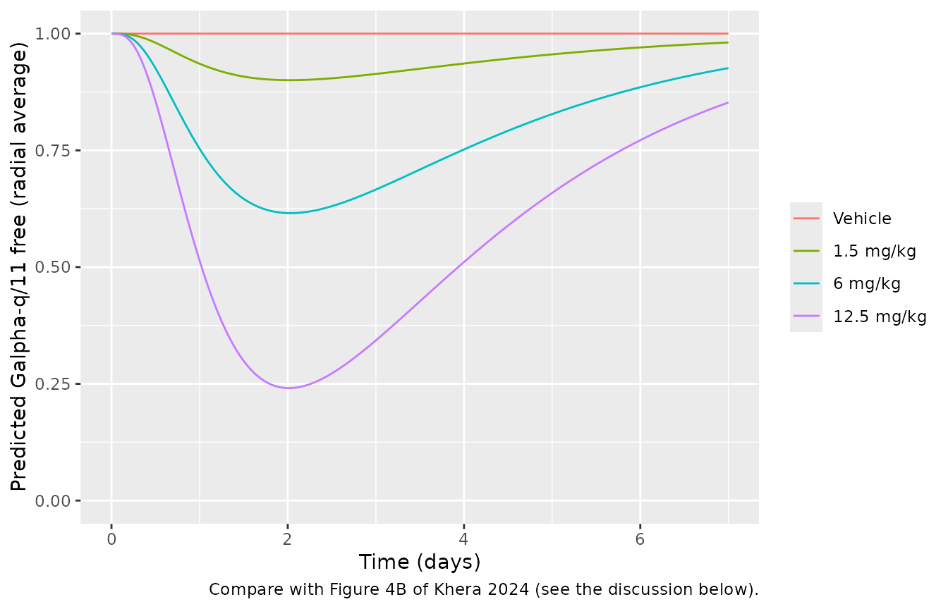
The Krogh model resolves the tumour radially around one capillary. The paper solves partial differential equations in MATLAB; the packaged model uses a method-of-lines discretisation into 10 equal-width shells. While building the model the maintainers solved the same equations with 5, 10, 20 and 40 shells (single doses, 20 g mouse, 150 kDa ADC); the minimum radial-average free Galpha-q/11 and the peak PMEL17 occupancy changed by at most 0.5% between 10 and 40 shells:
| Shells | Min. free Galpha-q/11, 1.5 / 6 / 12.5 mg/kg | Peak PMEL17 occupancy, 1.5 / 6 / 12.5 mg/kg |
|---|---|---|
| 5 | 0.9009 / 0.6164 / 0.2407 | 0.0716 / 0.2744 / 0.5395 |
| 10 | 0.9004 / 0.6157 / 0.2409 | 0.0719 / 0.2747 / 0.5388 |
| 20 | 0.9004 / 0.6158 / 0.2415 | 0.0719 / 0.2745 / 0.5381 |
| 40 | 0.9004 / 0.6161 / 0.2421 | 0.0718 / 0.2742 / 0.5376 |
mod_krogh <- readModelDb("Khera_2024_dyp688_mouse_krogh_qsp")
krogh_ev <- function(mgkg) {
  ev <- rxode2::et(seq(0, 168, by = 1))
  if (mgkg > 0) {
    amt <- mgkg_to_nmol(mgkg, wt_mouse)
    ev <- ev |>
      rxode2::et(amt = amt, cmt = "dar2_central") |>
      rxode2::et(amt = amt, cmt = "dar1_central") |>
      rxode2::et(amt = amt, cmt = "dar0_central")
  }
  ev
}
sim_krogh <- bind_rows(lapply(c(0, 1.5, 6, 12.5), function(d) {
  rxode2::rxSolve(mod_krogh, events = krogh_ev(d), returnType = "data.frame") |>
    mutate(dose = if (d == 0) "Vehicle" else paste(d, "mg/kg"))
})) |>
  mutate(dose = factor(dose, levels = c("Vehicle", "1.5 mg/kg", "6 mg/kg", "12.5 mg/kg")))

# Without drug the tumour stays at its baseline: surface PMEL17 at [Ag]0 and
# Galpha-q/11 fully free. This is an exact property of the equations, so the
# tolerance is numerical.
veh <- sim_krogh |> filter(dose == "Vehicle")
stopifnot(
  max(abs(veh$gq_free_frac - 1)) < 1e-6,
  max(abs(veh$target_free_slab5 - 83.3)) < 1e-6
)

ggplot(sim_krogh, aes(time / 24, gq_free_frac, colour = dose)) +
  geom_line() +
  coord_cartesian(ylim = c(0, 1)) +
  labs(
    x = "Time (days)", y = "Predicted Galpha-q/11 free (radial average)", colour = NULL,
    caption = "Compare with Figure 4B of Khera 2024 (see the discussion below)."
  )
sim_krogh |>
  filter(dose != "Vehicle") |>
  group_by(dose) |>
  summarise(
    `Minimum Galpha-q/11 free` = signif(min(gq_free_frac), 2),
    `Time of minimum (h)` = time[which.min(gq_free_frac)],
    `Peak PMEL17 occupancy` = signif(max(pmel17_occupancy), 2),
    .groups = "drop"
  ) |>
knitr::kable(caption = "Krogh model summary by single dose (20 g mouse, nominal 150 kDa ADC).")| dose | Minimum Galpha-q/11 free | Time of minimum (h) | Peak PMEL17 occupancy |
|---|---|---|---|
| 1.5 mg/kg | 0.90 | 49 | 0.072 |
| 6 mg/kg | 0.62 | 49 | 0.270 |
| 12.5 mg/kg | 0.24 | 48 | 0.540 |
Agreement with Figure 4B. The model reproduces the qualitative pattern of Figure 4B and Figure 4C: inhibition of Galpha-q/11 deepens and lasts longer as the dose rises, and recovers over days as Galpha-q/11 turns over. It does not reproduce the depth or the speed. Figure 4B shows about 50% free Galpha-q/11 at 1.5 mg/kg about 1.5 days after dosing, and near-complete inhibition at 6 and 12.5 mg/kg within the first day; the packaged model, with the Supplementary Table 1 parameters as printed, predicts roughly 90%, 60% and 25% free at about 2 days. The shortfall sits in ADC delivery, not in payload binding. With the printed antibody permeability (3 x 10^-9 m/s) the capillary supplies at most about 2 R_cap P_ADC / R_Krogh^2 = 0.017 per hour of the plasma concentration. That is a typical antibody tumour uptake, but it is several-fold below the payload delivery that Figure 4B implies. The chunk below repeats the simulation with a 10-fold higher antibody permeability, as a diagnostic only: 6 and 12.5 mg/kg then reach near-complete inhibition within about 1.5 days, as in Figure 4B, but 1.5 mg/kg overshoots the figure’s 50%. No single change to the exchange term reproduces all three curves, so the difference between the printed equations and the authors’ MATLAB implementation could not be traced. The paper does not give the plasma input, mouse weight or ADC mass used for these simulations. The packaged parameters are kept as published.
sim_krogh_p10 <- bind_rows(lapply(c(1.5, 6, 12.5), function(d) {
  rxode2::rxSolve(mod_krogh, events = krogh_ev(d), params = c(p_ab = 3e-8), returnType = "data.frame") |>
    mutate(dose = paste(d, "mg/kg"))
})) |>
  mutate(dose = factor(dose, levels = c("1.5 mg/kg", "6 mg/kg", "12.5 mg/kg")))
sim_krogh_p10 |>
  group_by(dose) |>
  summarise(
    `Minimum Galpha-q/11 free` = signif(min(gq_free_frac), 2),
    `Time of minimum (h)` = time[which.min(gq_free_frac)],
    .groups = "drop"
  ) |>
knitr::kable(caption = "Diagnostic only: Krogh model with P_ADC = 3 x 10^-8 m/s (10-fold the published value).")| dose | Minimum Galpha-q/11 free | Time of minimum (h) |
|---|---|---|
| 1.5 mg/kg | 0.3200 | 49 |
| 6 mg/kg | 0.0091 | 36 |
| 12.5 mg/kg | 0.0072 | 35 |
Assumptions and deviations
-
Dose entry. The authors’ Monolix models split each
dose between the three ADC species through three
depot()targets. Here every dose is three records of the same nmol amount, one into each ofdar2_central,dar1_centralanddar0_central;f()applies the split. Infusions must usedur, notrate, so thatf()scales the infused amount. - Masses for the simulations. The paper does not state the ADC molecular weight or the animals’ body weights. The simulations here assume 150 kDa for the ADC, 20 g for a nude mouse, and the paper’s own 3 kg and 70 kg for monkey and human; FR900359 is 1000 g/mol (Supplementary Table 1). The models themselves take doses in nmol and are unaffected. The resulting peak active payload concentrations in mice match the Cmax axis of Figure 3B.
-
Concentration units. The Monolix description gives
mouse doses in nmol and volume in mL, while the fitted concentrations
and
kkillare in nM. The mouse models therefore report1000 * amount / Vc(nM), which is what makeskkill(1/nM/h) and the tumorostatic concentrations of Table 4 consistent. - Mouse residual errors. Table 1 lists the log-scale residual errors as 0.41 (total antibody), 0.24 (active ADC) and 0.52 (inactive ADC). The Monolix output in the Supplementary Material ties the same three numbers to its observation IDs differently: 0.518 for total antibody, 0.409 for active ADC and 0.244 for inactive ADC. The model follows the Monolix output.
- IIV on tumour growth. The vehicle Gompertz fit had IIV on beta (SD 0.456) and TSmax (SD 0.255; Table 3). The Monolix PK-TGI run that gives the final drug-effect estimates has no random effect on either (every individual beta and TSmax equals the population value), so the TGI model has none. The vehicle-fit residual SD (0.148) is likewise superseded by the PK-TGI value (0.734).
- Rounded PK in the TGI model. The PK-TGI run held the PK at Table 1 values rounded to two significant figures (for example kel 0.016, TSmax 929); the TGI model uses those, while the stand-alone mouse PK model uses the full-precision estimates.
-
Dose levels outside the fit.
DOSE_DYP688_MGKGvalues other than 3 or 6 mg/kg use the reference (1.5 mg/kg) kill rate, the conservative choice the authors made for their subsequent simulations. - FcRn-mut residual error. Supplementary Table 2 does not report residual error for the FcRn-mut fit; the DYP688 mouse values (same model, same assays) are carried over and fixed.
- Human variability and residual error. The human projection has no fitted variability. Table 5 reports the human interquartile ranges as the monkey ranges scaled, so the monkey IIV (V, k21, ki.a.) and residual errors are carried over and fixed.
- Human elimination rate. Table 5 gives CL and Vc; the model uses kel = CL / Vc = 0.0251 / 1.93 1/h and an inactivation rate of ln 2 / 61 h.
- Krogh model discretisation. See the Krogh section: 10 radial shells, the payload capillary boundary uses the antibody void fraction epsilon as printed (epsilon (1 + R)), and the radial averages are unweighted means over the equal-width shells.
-
Supplementary Table 1 unit typos. k_off,P is
printed in M^-1 s^-1 and the partition coefficient R in m/s; they are
used as s^-1 and dimensionless. The printed central-compartment equation
for ADC0P has
k12 ADC1P,cwhere the Monolix code hask12 * ADC_0P_C; the code is used. - No erratum or correction notice for this article was found as of 2026-11-01.