Physiologically-inspired PKRO of dupilumab (Kapitanov 2025)
Source:vignettes/articles/Kapitanov_2025_dupilumab.Rmd
Kapitanov_2025_dupilumab.RmdOverview
Kapitanov et al. 2025 introduce a physiologically-inspired PKRO
(piPKRO) model class for monoclonal antibodies. The framework
reparameterises the classical two-compartment PK model with (a) drug
elimination in every compartment, (b) a physiological peripheral volume
fixed at the total body interstitial volume, and (c) three
macroparameters – the linear elimination half-life t_half,
the central-peripheral distribution half-time t_dist, and
the peripheral partition coefficient P_dist – in place of
clearance / inter-compartmental clearance. Adding mass-action
full-binding TMDD in every compartment yields the piPKRO model. Case
studies fit and simulate the model for dupilumab, an
anti-interleukin-4-receptor (IL4R) IgG4 antibody used in atopic
dermatitis.
This vignette walks the paper’s three case studies:
- Case Study 1 – Bottom-up prediction with standard mAb parameters (no fit; Kapitanov 2025 Figure 3).
-
Case Study 2 – Calibration of the 2-compartment
piPKRO to digitised single-dose dupilumab PK in healthy volunteers
(Kapitanov 2025 Figure 4). Packaged model:
Kapitanov_2025_dupilumab_qsp. -
Case Study 3 Approach 2 – Extension to a
3-compartment piPKRO with a skin site-of-action (SoA) compartment
(Kapitanov 2025 Figure 5). Packaged model:
Kapitanov_2025_dupilumab_3cmt_qsp.
Model and source
- Packaged 2-cpt model:
Kapitanov_2025_dupilumab_qsp - Packaged 3-cpt model:
Kapitanov_2025_dupilumab_3cmt_qsp - Article: CPT: Pharmacometrics & Systems Pharmacology 10.1002/psp4.70160
- Case Study 2 upstream dupilumab PK: Li E et al. J Clin Pharmacol 2015 (Kapitanov 2025 ref 35; observed data digitised for calibration).
Population
The clinical PK data in Case Studies 2 and 3 come from the dupilumab first-in-human single-ascending-dose study of Li 2015 (Kapitanov 2025 ref 35): healthy adult volunteers receiving single intravenous doses of 1, 3, 8, or 12 mg/kg dupilumab. Kapitanov 2025 does not report a per-subject fit or population variance for the case studies – the paper reports typical values only for the linear-PK-related parameters after calibration to digitised mean PK profiles. IL4R target concentrations in the central (0.00605 nM) and peripheral (0.127 nM) compartments come from a bottom-up cell-count sum per Marcantonio et al. 2020 (Kapitanov 2025 ref 34) tabulated in Kapitanov 2025 Table S5. The Case Study 3 SoA compartment represents inflamed atopic-dermatitis skin (indication for dupilumab) with an elevated bottom-up IL4R concentration of 2.02 nM reflecting the higher immune-cell infiltrate and per-cell IL4R expression in inflamed skin.
The population metadata for each model is available
programmatically:
readModelDb("Kapitanov_2025_dupilumab_qsp")()$population
#> $species
#> [1] "human"
#>
#> $n_subjects
#> [1] NA
#>
#> $n_studies
#> [1] 1
#>
#> $age_range
#> [1] "healthy adult volunteers"
#>
#> $weight_range
#> [1] "assumed 70 kg for the deterministic simulation"
#>
#> $weight_median
#> [1] "70 kg (Kapitanov 2025 Section 2.4 standard human)"
#>
#> $sex_female_pct
#> [1] NA
#>
#> $race_ethnicity
#> [1] NA
#>
#> $disease_state
#> [1] "Healthy adult volunteers from the dupilumab first-in-human single-ascending-dose IV study reported in Li E et al. 2015 (Kapitanov 2025 ref 35). Mean PK profiles at 1, 3, 8, and 12 mg/kg were digitised from Li 2015 for the Case Study 2 fit."
#>
#> $dose_range
#> [1] "Single IV bolus at 1, 3, 8, and 12 mg/kg (70, 210, 560, 840 mg at 70 kg)."
#>
#> $regions
#> [1] NA
#>
#> $notes
#> [1] "Kapitanov 2025 does not perform a per-subject fit for Case Study 2; the paper reports only typical values of the linear PK-related parameters after calibration to digitised mean PK profiles. No IIV / OMEGA and no residual-error / SIGMA are reported. The IL4R central and peripheral target concentrations (C_R,1 = 0.00605 nM, C_R,2 = 0.127 nM) were held fixed at the bottom-up estimates from Kapitanov 2025 Table S5 (Marcantonio 2020 methodology)."
Source trace
Per-parameter provenance is recorded as an in-file comment next to
each ini() entry in
inst/modeldb/specificDrugs/Kapitanov_2025_dupilumab_qsp.R
and Kapitanov_2025_dupilumab_3cmt_qsp.R. The following
table summarises the source of every equation and every fitted / fixed
parameter value across the three case studies.
| Equation / parameter | Value | Source location |
|---|---|---|
| piPK model definition (Eqs 3-4) | n/a | Kapitanov 2025 Section 2.1, Eqs 3-4 |
| macroparameter conversion (Eqs 5-7) | n/a | Kapitanov 2025 Section 2.1, Eqs 5-7 |
| 3-cpt piPK extension (Eqs 9-10) | n/a | Kapitanov 2025 Section 2.3, Eqs 9-10 |
| full-binding TMDD ODEs (Eqs 11-16) | n/a | Kapitanov 2025 Section 2.3, Eqs 11-16 |
| target synthesis (Eq 23) | n/a | Kapitanov 2025 Section 2.4, Eq 23 |
| 3-cpt t_dist adjustment (Eqs 21-22) | n/a | Kapitanov 2025 Section 2.4, Eqs 21-22 |
| standard mAb V_1 | 3.24 L | Kapitanov 2025 Table 2 (Case 1) |
| standard mAb V_2 | 13 L | Kapitanov 2025 Table 2 (Case 1) |
| standard mAb t_half | 16.5 d | Kapitanov 2025 Table 2 (Case 1) |
| standard mAb t_dist | 49 h | Kapitanov 2025 Table 2 (Case 1) |
| standard mAb P_dist | 0.267 | Kapitanov 2025 Table 2 (Case 1) |
| fitted 2-cpt V_1 | 2.29 L | Kapitanov 2025 Table S4 (Case 2 fitted) |
| fitted 2-cpt V_2 | 12.4 L | Kapitanov 2025 Table S4 (Case 2 fitted) |
| fitted 2-cpt t_half | 32.8 d | Kapitanov 2025 Table S4 (Case 2 fitted) |
| fitted 2-cpt t_dist,12 | 54.3 h | Kapitanov 2025 Table S4 (Case 2 fitted) |
| fitted 2-cpt P_dist,12 | 0.352 | Kapitanov 2025 Table S4 (Case 2 fitted) |
| 3-cpt t_dist,12 (recomputed) | 55.9 h | Kapitanov 2025 Table S4 (Case 3 via Eq 22) |
| 3-cpt V_3 (SoA / skin) | 0.563 L | Kapitanov 2025 Table S4 (50% of 1.125 L interstitial skin) |
| 3-cpt Approach 2 t_dist,13 | 30 h | Kapitanov 2025 Table S4 (Case 3 Approach 2) |
| 3-cpt Approach 2 P_dist,13 | 0.3 | Kapitanov 2025 Table S4 (Case 3 Approach 2) |
| central IL4R C_R,1 | 0.00605 nM | Kapitanov 2025 Table S4 and Table S5 (bottom-up) |
| peripheral IL4R C_R,2 | 0.127 nM | Kapitanov 2025 Table S4 and Table S5 (bottom-up) |
| SoA IL4R C_R,3 (inflamed skin) | 2.02 nM | Kapitanov 2025 Table S4 and Table S5 (bottom-up) |
| IL4R k_deg | 1 /h | Kapitanov 2025 Table S4 and Section 3.1 (from ref 40, Andrews et al.) |
| Dupilumab-IL4R k_on | 1e-3 /(nM*s) | Kapitanov 2025 Table S4 (K_D = 33 pM per ref 41, Kuo 2010) |
| Dupilumab-IL4R k_off | 3.3e-5 /s | Kapitanov 2025 Table S4 (with k_on gives K_D = 33 pM) |
| Complex degradation rate | k_deg (same as free target) | Kapitanov 2025 Section 3.1 |
The dupilumab MW is assumed at the standard human IgG4 value of 147 kDa (147000 g/mol); Kapitanov 2025 does not state MW explicitly, but Figure 4’s y-axis in ug/mL (= mg/L) implies the authors used a standard IgG4 MW for their reported mass-based observed data.
Case Study 1 – Bottom-up PK prediction with standard mAb parameters
Kapitanov 2025 Section 3.1 demonstrates that a piPKRO model built
from standard-mAb typical parameter values (Table 2) plus a bottom-up
IL4R target burden reasonably predicts dupilumab nonlinear PK
without any fit. In particular, the standard-parameter
model captures the faster clearance at 1 mg/kg (TMDD dominant) while
under-predicting exposure at the higher doses. The 2-compartment piPKRO
packaged as Kapitanov_2025_dupilumab_qsp uses the Case
Study 2 fitted parameters; to reproduce Case Study 1 we override the
fitted structural parameters back to the standard values from Kapitanov
2025 Table 2 using nlmixr2est::ini.
mod2 <- readModelDb("Kapitanov_2025_dupilumab_qsp")

# Case Study 1 = standard mAb piPK parameters (Kapitanov 2025 Table 2)
mod_case1 <- rxode2::ini(mod2,
  lvc    = log(3.24),
  lvp    = log(13),
  lthalf = log(16.5 * 24),  # 16.5 d in hours
  ltdist = log(49),
  lpdist = log(0.267)
)
Simulate a single IV bolus at each of 1, 3, 8, 12 mg/kg (70 kg body weight assumed):
make_iv_events <- function(dose_mg_per_kg, bw = 70, cmt = "central",
                           t_end_h = 60 * 24) {
  amt <- dose_mg_per_kg * bw
  ev <- rxode2::et(amt = amt, cmt = cmt) |>
    rxode2::et(seq(0, t_end_h, by = 4))
  as.data.frame(ev) |>
    dplyr::mutate(treatment = sprintf("%s mg/kg", dose_mg_per_kg))
}
doses_mg_per_kg <- c(1, 3, 8, 12)

events_case1 <- lapply(seq_along(doses_mg_per_kg), function(i) {
  make_iv_events(doses_mg_per_kg[i]) |>
    dplyr::mutate(id = i)
}) |>
  dplyr::bind_rows()

sim_case1 <- rxode2::rxSolve(mod_case1, events = events_case1,
                             keep = "treatment") |>
  as.data.frame() |>
  dplyr::mutate(time_d = time / 24)
Replicate the shape of Kapitanov 2025 Figure 3a-c (central PK, central RO, peripheral RO):
sim_case1 |>
  ggplot(aes(time_d, Cc, colour = treatment, group = treatment)) +
  geom_line(linewidth = 0.8) +
  scale_y_log10() +
  labs(x = "Time (days)", y = "Central dupilumab (mg/L)",
       title = "Case Study 1 - Figure 3a",
       colour = "Dose",
       caption = "Replicates the shape of Kapitanov 2025 Figure 3a using the standard-mAb parameters of Table 2.")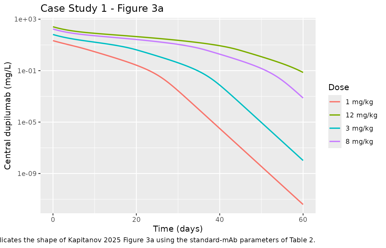
Case Study 1: central dupilumab concentration-time profile at 1, 3, 8, 12 mg/kg IV; standard-mAb parameters + bottom-up IL4R burden.
sim_case1 |>
  dplyr::select(time_d, treatment, `Central` = RO_c, `Peripheral` = RO_p) |>
  tidyr::pivot_longer(cols = c("Central", "Peripheral"),
                      names_to = "compartment", values_to = "RO") |>
  ggplot(aes(time_d, 100 * RO, colour = treatment, group = treatment)) +
  geom_line(linewidth = 0.8) +
  facet_wrap(~compartment, ncol = 1) +
  labs(x = "Time (days)", y = "RO (%)",
       title = "Case Study 1 - Figure 3b/c",
       colour = "Dose",
       caption = "Replicates the shape of Kapitanov 2025 Figure 3b (central RO) and 3c (peripheral RO).")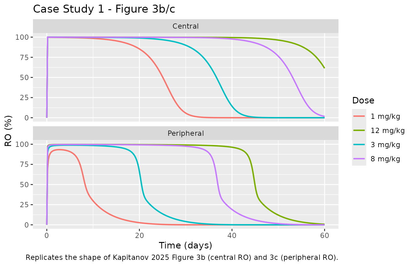
Case Study 1: receptor occupancy in central (top) and peripheral (bottom) compartments.
Case Study 2 – Calibrated 2-compartment piPKRO
Case Study 2 calibrates the linear-PK-related parameters
(V_1, V_2, t_half,
t_dist,12, P_dist,12) to digitised mean
concentration-time profiles from Li 2015; the target and binding
parameters are held at the same bottom-up / literature values as Case 1.
The Kapitanov_2025_dupilumab_qsp model carries the fitted
parameter set as its defaults.
mod_case2 <- readModelDb("Kapitanov_2025_dupilumab_qsp")
sim_case2 <- rxode2::rxSolve(mod_case2, events = events_case1,
                             keep = "treatment") |>
  as.data.frame() |>
  dplyr::mutate(time_d = time / 24)
Replicate Kapitanov 2025 Figure 4a-c:
sim_case2 |>
  ggplot(aes(time_d, Cc, colour = treatment, group = treatment)) +
  geom_line(linewidth = 0.8) +
  scale_y_log10() +
  labs(x = "Time (days)", y = "Central dupilumab (mg/L)",
       title = "Case Study 2 - Figure 4a",
       colour = "Dose",
       caption = "Replicates the shape of Kapitanov 2025 Figure 4a (calibrated 2-cpt piPKRO).")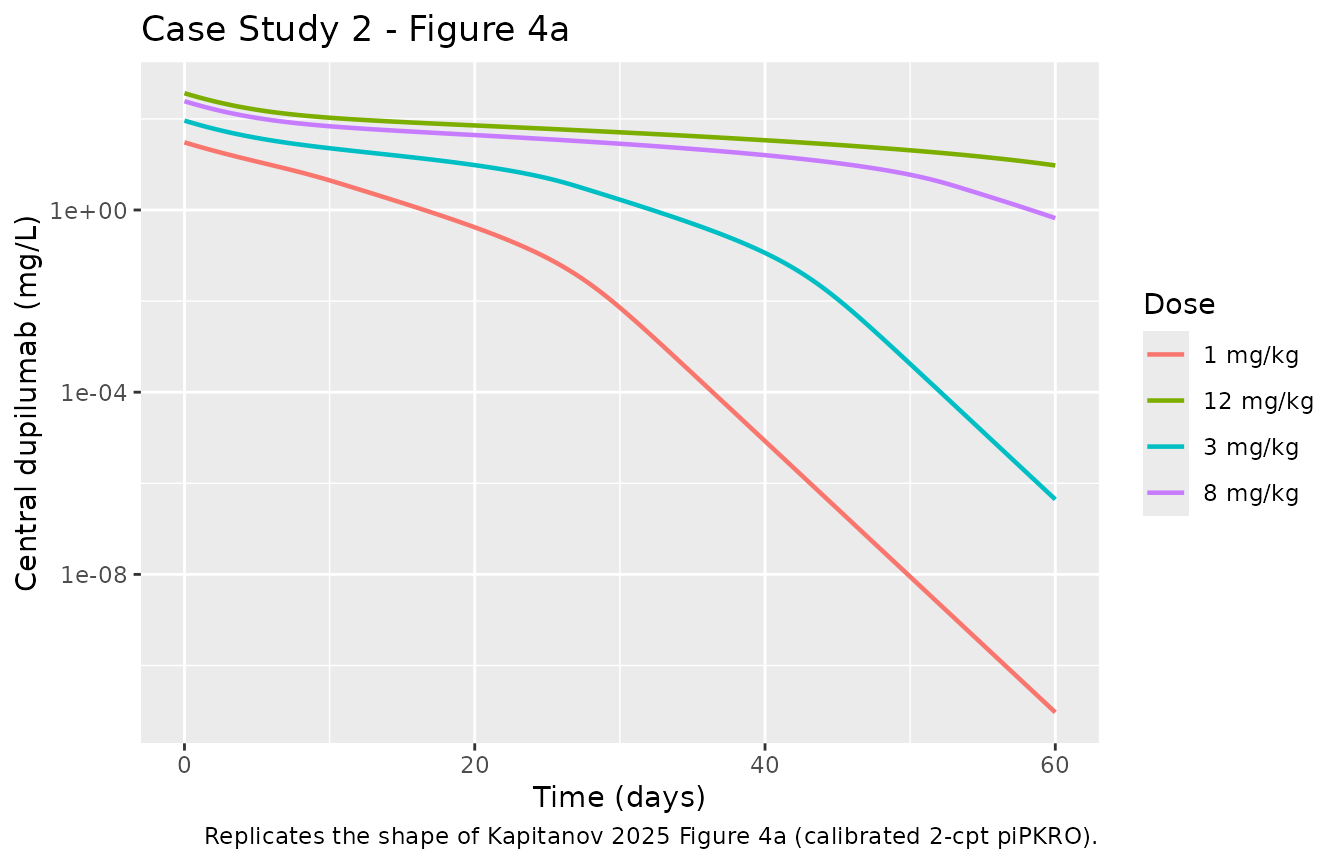
Case Study 2: central dupilumab concentration-time profile at 1, 3, 8, 12 mg/kg IV; 2-compartment piPKRO with fitted linear-PK parameters.
sim_case2 |>
  dplyr::select(time_d, treatment, `Central` = RO_c, `Peripheral` = RO_p) |>
  tidyr::pivot_longer(cols = c("Central", "Peripheral"),
                      names_to = "compartment", values_to = "RO") |>
  ggplot(aes(time_d, 100 * RO, colour = treatment, group = treatment)) +
  geom_line(linewidth = 0.8) +
  facet_wrap(~compartment, ncol = 1) +
  labs(x = "Time (days)", y = "RO (%)",
       title = "Case Study 2 - Figure 4b/c",
       colour = "Dose",
       caption = "Replicates the shape of Kapitanov 2025 Figure 4b (central RO) and 4c (peripheral RO).")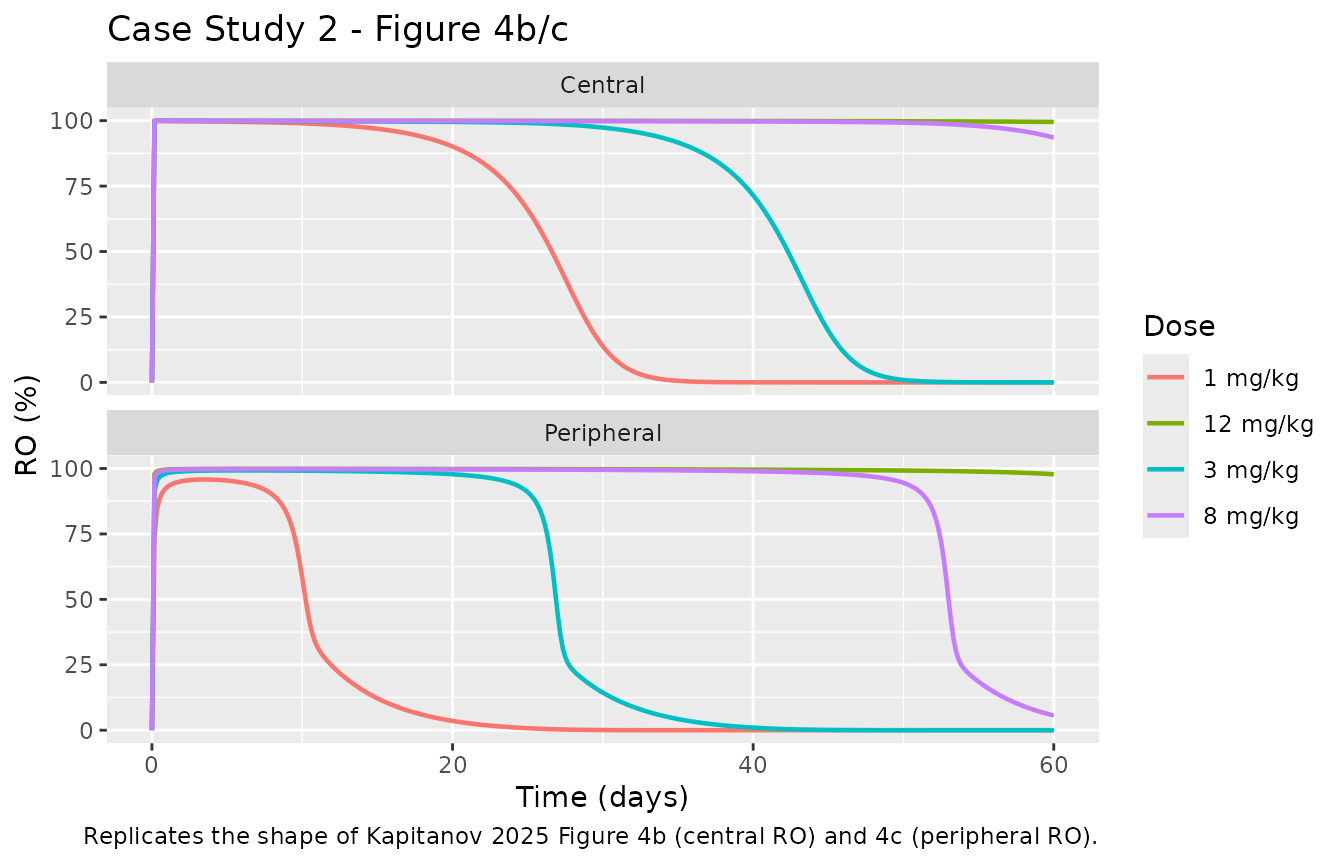
Case Study 2: receptor occupancy in central (top) and peripheral (bottom) compartments after calibration.
Comparison of Case Study 1 (bottom-up prediction) and Case Study 2 (calibrated fit) at the highest dose:
dplyr::bind_rows(
  sim_case1 |> dplyr::filter(treatment == "12 mg/kg") |>
    dplyr::mutate(case = "Case 1 (standard mAb params)"),
  sim_case2 |> dplyr::filter(treatment == "12 mg/kg") |>
    dplyr::mutate(case = "Case 2 (fitted)")
) |>
  ggplot(aes(time_d, Cc, colour = case, group = case)) +
  geom_line(linewidth = 0.8) +
  scale_y_log10() +
  labs(x = "Time (days)", y = "Central dupilumab (mg/L)",
       title = "12 mg/kg IV: Case Study 1 vs Case Study 2",
       colour = NULL)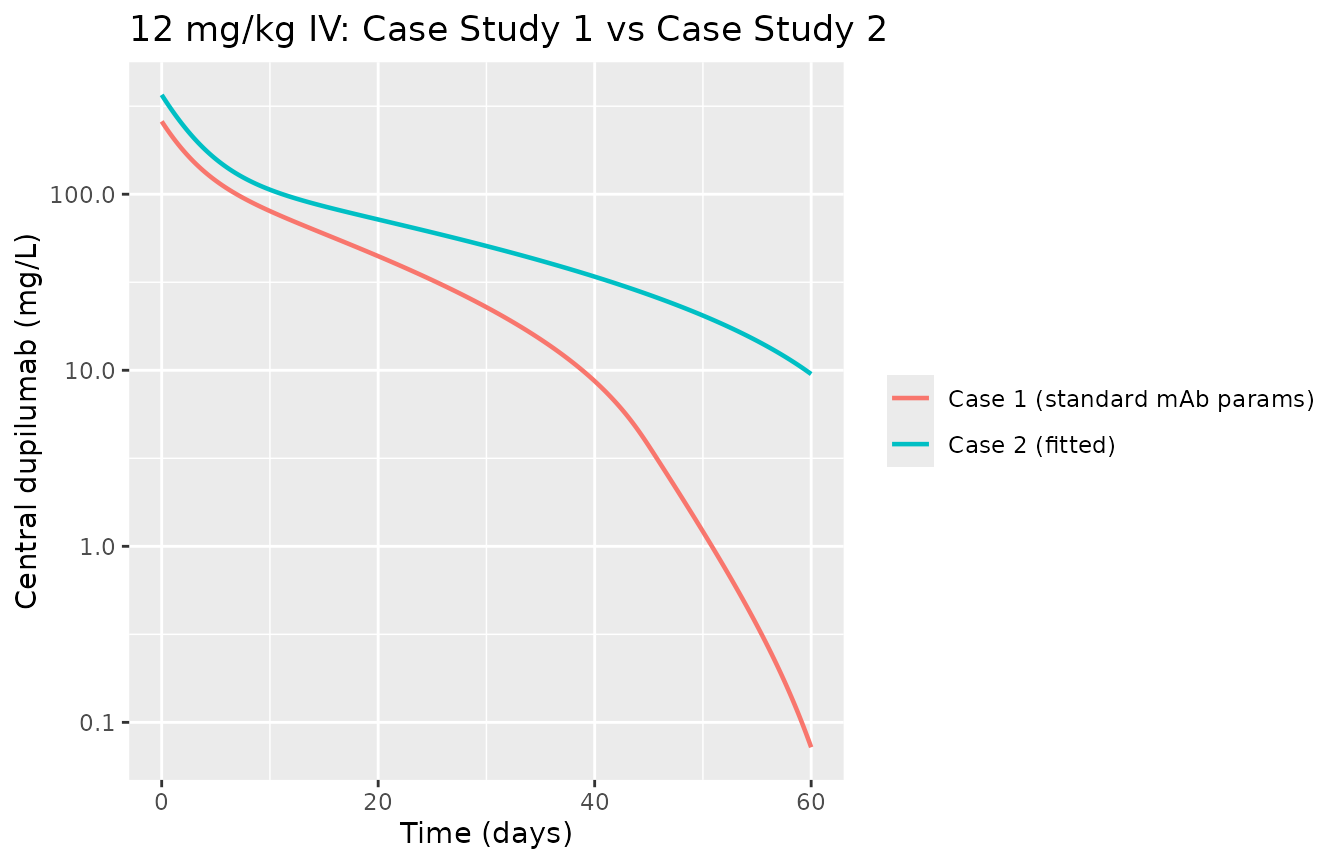
Case Study 1 vs Case Study 2 at 12 mg/kg IV. Fitted PK produces the higher observed exposure; Case 1 under-predicts.
Case Study 3 Approach 2 – 3-compartment piPKRO with a skin SoA
Case Study 3 adds a third compartment representing 50% of the total
interstitial skin volume (0.563 L) as a site of action for dupilumab in
inflamed atopic-dermatitis skin. Approach 2 (packaged as
Kapitanov_2025_dupilumab_3cmt_qsp) fixes the central-to-SoA
distribution half-time t_dist,13 = 30 h and the SoA
partition coefficient P_dist,13 = 0.3 (representing a lower
ratio than the lumped peripheral, reflecting the tighter skin barrier).
The SoA IL4R concentration is set to 2.02 nM based on the bottom-up
cell-count sum for inflamed skin (Kapitanov 2025 Table S5).
mod_case3 <- readModelDb("Kapitanov_2025_dupilumab_3cmt_qsp")
events_case3 <- lapply(seq_along(doses_mg_per_kg), function(i) {
  make_iv_events(doses_mg_per_kg[i], t_end_h = 60 * 24) |>
    dplyr::mutate(id = i)
}) |>
  dplyr::bind_rows()

sim_case3 <- rxode2::rxSolve(mod_case3, events = events_case3,
                             keep = "treatment") |>
  as.data.frame() |>
  dplyr::mutate(time_d = time / 24)
Replicate Kapitanov 2025 Figure 5a (central PK) and 5b-d (RO in central, peripheral, and SoA):
sim_case3 |>
  ggplot(aes(time_d, Cc, colour = treatment, group = treatment)) +
  geom_line(linewidth = 0.8) +
  scale_y_log10() +
  labs(x = "Time (days)", y = "Central dupilumab (mg/L)",
       title = "Case Study 3 Approach 2 - Figure 5a",
       colour = "Dose",
       caption = "Replicates the shape of Kapitanov 2025 Figure 5a (3-cpt piPKRO Approach 2 solid lines).")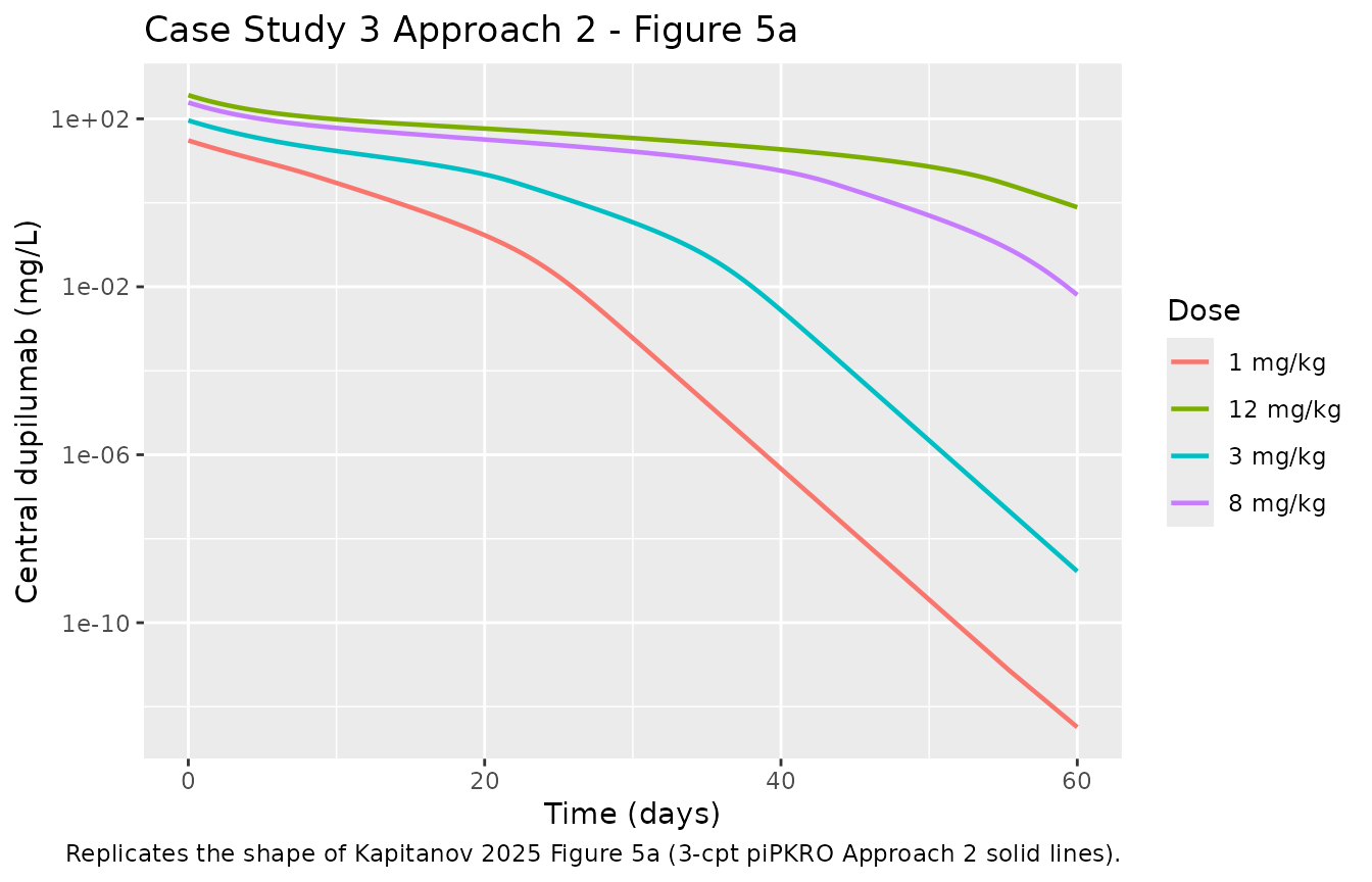
Case Study 3 Approach 2: central dupilumab concentration-time profile at 1, 3, 8, 12 mg/kg IV.
sim_case3 |>
  dplyr::select(time_d, treatment,
                `Central`    = RO_c,
                `Peripheral` = RO_p,
                `SoA (skin)` = RO_soa) |>
  tidyr::pivot_longer(cols = c("Central", "Peripheral", "SoA (skin)"),
                      names_to = "compartment", values_to = "RO") |>
  dplyr::mutate(compartment = factor(compartment,
                                     levels = c("Central", "Peripheral", "SoA (skin)"))) |>
  ggplot(aes(time_d, 100 * RO, colour = treatment, group = treatment)) +
  geom_line(linewidth = 0.8) +
  facet_wrap(~compartment, ncol = 1) +
  labs(x = "Time (days)", y = "RO (%)",
       title = "Case Study 3 Approach 2 - Figure 5b/c/d",
       colour = "Dose",
       caption = "Replicates the shape of Kapitanov 2025 Figure 5b (central), 5c (peripheral), and 5d (SoA / skin).")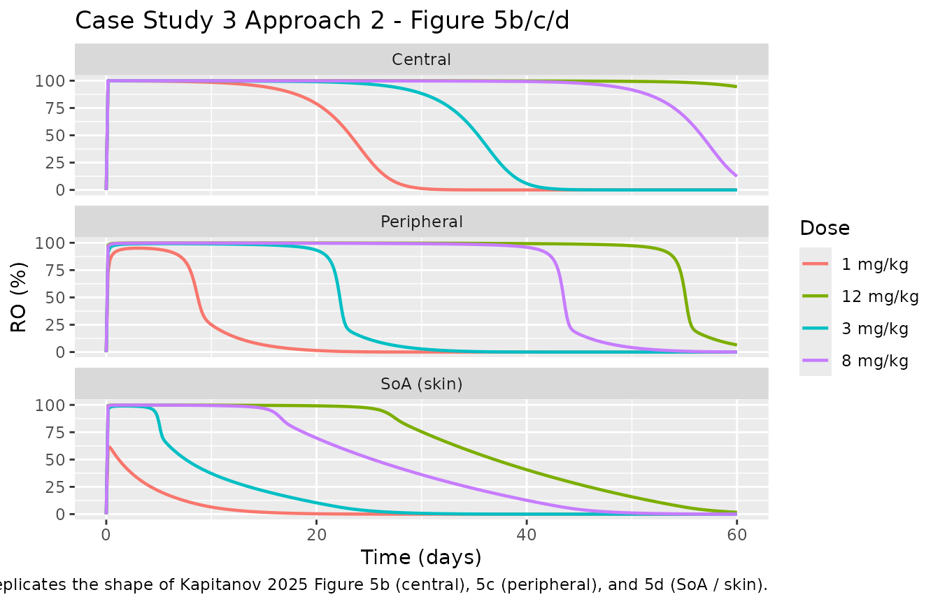
Case Study 3 Approach 2: receptor occupancy in central (top), peripheral (middle), and SoA / skin (bottom) compartments. The SoA RO is markedly lower than central and peripheral RO for all but the highest doses – the paper’s local drug depletion effect.
Validation sanity checks
Central-compartment concentration matches classical 2-cpt PK
In the absence of TMDD, the piPK 2-cpt model must produce the same central-compartment concentration profile as a classical 2-cpt PK model with the equivalent CL / Q / V1 / V2 (Kapitanov 2025 Section 2.1, Table S1). Set the target concentrations to a tiny value to effectively disable TMDD and observe first-order decay:
mod_case2_noTMDD <- rxode2::ini(mod2,
  lc_r_c = log(1e-12),
  lc_r_p = log(1e-12)
)
sim_linear <- rxode2::rxSolve(
  mod_case2_noTMDD,
  events = make_iv_events(12, t_end_h = 120 * 24) |>
    dplyr::mutate(id = 1L, treatment = "12 mg/kg no-TMDD")
) |>
  as.data.frame() |>
  dplyr::mutate(time_d = time / 24)

# At infinite time in the absence of TMDD, log(Cc) should decay
# linearly at slope -kel = -log(2) / t_half.
late <- sim_linear |> dplyr::filter(time_d >= 50)
fit_slope <- coef(lm(log(Cc) ~ time_d, data = late))
observed_thalf_d <- -log(2) / fit_slope[["time_d"]]
cat(sprintf(
  "Terminal-phase half-life (no TMDD): observed = %.2f d; encoded lthalf = %.2f d\n",
  observed_thalf_d, 32.8
))
#> Terminal-phase half-life (no TMDD): observed = 32.80 d; encoded lthalf = 32.80 d
The observed terminal-phase half-life matches the encoded
t_half macroparameter, consistent with the piPK framework’s
claim (Eq 8, Table 1) that k_el = beta = log(2) / t_half
when drug elimination occurs in both compartments.
Steady-state target concentration
Before drug administration the target free concentration in each
compartment should be exactly C_R,i. Confirm:
sim_ss <- sim_case2 |> dplyr::filter(time == 0)
cat("Central target free concentration at t=0 (nM):",
    format(unique(sim_ss$Cr_c), digits = 4), "\n")
#> Central target free concentration at t=0 (nM): 0.00605
cat("Peripheral target free concentration at t=0 (nM):",
    format(unique(sim_ss$Cr_p), digits = 4), "\n")
#> Peripheral target free concentration at t=0 (nM): 0.127
cat("Encoded C_R,1 = 0.00605 nM; C_R,2 = 0.127 nM\n")
#> Encoded C_R,1 = 0.00605 nM; C_R,2 = 0.127 nM
Dose linearity above the TMDD-saturating dose
At doses saturating TMDD, Cmax should scale linearly with dose. Extract peak central concentration by dose from Case Study 2:
cmax_summary <- sim_case2 |>
  dplyr::group_by(treatment) |>
  dplyr::summarise(Cmax_mgL = max(Cc, na.rm = TRUE), .groups = "drop") |>
  dplyr::mutate(dose_mg = as.numeric(gsub(" mg/kg", "", treatment)) * 70,
                Cmax_per_mg = Cmax_mgL / dose_mg)

cmax_summary |>
  dplyr::rename(`Dose group` = treatment,
                `Cmax (mg/L)` = Cmax_mgL,
                `Dose (mg)`   = dose_mg,
                `Cmax / dose (mg/L per mg)` = Cmax_per_mg) |>
  knitr::kable(digits = c(0, 2, 0, 4),
caption = "Peak central concentration by IV dose. Cmax/dose is approximately constant across doses because bolus IV Cmax is dominated by V_1 and independent of TMDD (which acts on the decline phase).")| Dose group | Cmax (mg/L) | Dose (mg) | Cmax / dose (mg/L per mg) |
|---|---|---|---|
| 1 mg/kg | 30.57 | 70 | 0.4367 |
| 12 mg/kg | 366.81 | 840 | 0.4367 |
| 3 mg/kg | 91.70 | 210 | 0.4367 |
| 8 mg/kg | 244.54 | 560 | 0.4367 |
Assumptions and deviations
- Dupilumab molecular weight: The paper does not state the MW explicitly; the standard human IgG4 monoclonal-antibody value of 147 kDa (147000 g/mol) is used here for the mg/L <-> nM conversion. Kapitanov 2025 Figure 4 y-axis (Concentration [ug/mL]) implies the authors used a standard IgG4 MW for their reported observed data.
- No IIV / no residual error: Kapitanov 2025 Case Studies 2 and 3 are deterministic single-subject fits to digitised mean PK profiles; the paper reports typical values only, with no OMEGA and no SIGMA. Both packaged model files are encoded without IIV / residual error.
-
k_deg unit interpretation: Kapitanov 2025 Table S4
lists
k_degwith units ofhand value1. Section 3.1 text says “the elimination rate of IL4R was fixed to be 1 h [ref 40]”. This is interpreted here as a first-order rate constant of magnitude 1 with units1/h(i.e., IL4R turnover half-life = log(2) h approximately 42 min), matching the table’s face value. An alternative reading (“half-life = 1 h”, rate constant = log(2)/h) would yield a slightly slower receptor turnover but preserve the qualitative behaviour. - Case Study 3 peripheral volume: Kapitanov 2025 Section 3.3 says “the volume of the peripheral compartment was decreased by subtracting the SoA compartment volume”, but Table S4 Approach 2 reports V_2 = 12.4 L, identical to Case 2, without subtracting V_3 = 0.563 L. This file follows Table S4 (the authoritative parameter table) verbatim; the resulting total peripheral + SoA volume is 12.963 L instead of 12.4 L (about 4 percent higher than Case 2’s lumped peripheral).
-
Case Study 1 vs Case Study 2: The packaged
Kapitanov_2025_dupilumab_qspmodel carries the Case Study 2 fitted parameters as its defaults. Case Study 1 (bottom-up prediction with standard mAb parameters) is reproduced in this vignette via a parameter override (rxode2::ini(mod, ...)) rather than as a separate model file, because the two cases differ only in the values of 5 structural parameters and share the same ODE / target binding structure. -
Case Study 3 Approach 1 not packaged: The paper’s
Case Study 3 Approach 1 (assuming the SoA drug profile equals the
peripheral profile, with
t_dist,13 = 150 hcomputed via Eq 22) is not packaged as a separate file. Users interested in Approach 1 can simulate it with a parameter override onKapitanov_2025_dupilumab_3cmt_qsp(ltdist_p2 = log(150),lpdist_p2 = log(0.352)). - Bottom-up target burden: The IL4R central and peripheral target concentrations are computed by summing cell-count times per-cell IL4R expression times fraction-of-cells-expressing-target across the immune / stromal cell types in Kapitanov 2025 Table S5. The paper’s Section 3.1 notes that the assays are often qualitative rather than quantitative, so the bottom-up estimates are best interpreted as first-principles predictions rather than measured values.
-
This is a tutorial paper: Kapitanov 2025 is a
tutorial introducing the piPKRO modeling framework, not a de novo popPK
/ QSP model of dupilumab. Dupilumab popPK developed from Phase 3 data is
available as
Kovalenko_2016_dupilumab,Kovalenko_2020_dupilumab(base and covariate), andZhang_2021_dupilumabin this package. The piPKRO framework’s contribution is complementary: it provides a physiologically-inspired mechanistic backbone that can be used for dose prediction and target occupancy in tissues where popPK models are silent.