Riociguat (Michalickova 2020)
Source:vignettes/articles/Michalickova_2020_riociguat.Rmd
Michalickova_2020_riociguat.RmdModel and source
- Citation: Michalickova D, Jansa P, Bursova M, Hlozek T, Cabala R, Hartinger JM, Ambroz D, Aschermann M, Lindner J, Linhart A, Slanar O, Krekels EHJ. Population pharmacokinetics of riociguat and its metabolite in patients with chronic thromboembolic pulmonary hypertension from routine clinical practice. Pulm Circ. 2020;10(1):2045894019898031. doi:10.1177/2045894019898031. The absorption rate constant is fixed to a literature value (Michalickova 2020 ref 17: Saleh S, Becker C, Frey R, et al. Population pharmacokinetics of single-dose riociguat in patients with renal or hepatic impairment. Pulm Circ. 2016;6:S75-S85).
- Description: Joint parent (riociguat) + metabolite (M1, desmethylriociguat) population PK model in adults with chronic thromboembolic pulmonary hypertension (CTEPH) treated in routine clinical practice (Michalickova 2020). Riociguat is one-compartment with first-order absorption (ka fixed at 3 1/h from the literature) and two parallel first-order elimination routes from the central compartment: metabolic formation of M1 (CLf,M1/F, power function of total bilirubin centred at 0.69 mg/dL) and all remaining pathways (CLe,r/F, linear in creatinine clearance centred at 70 mL/min). M1 is one-compartment with first-order elimination (CLe,M1/F) and shares the parent’s apparent volume of distribution (assumed for identifiability). An absorption lag time of 2.95 h applies only to the six patients whose late post-dose concentrations were unexpectedly high (MIX_LAGGED_ABS = 1). With one sample per patient, inter-individual and residual variability could not be separated, so the model carries no etas and the proportional residual errors absorb both.
- Article: https://doi.org/10.1177/2045894019898031 (open access)
Riociguat is a soluble guanylate cyclase stimulator used for chronic thromboembolic pulmonary hypertension (CTEPH). Its main circulating metabolite, M1 (desmethylriociguat), is pharmacologically active. Michalickova 2020 fitted a joint parent + metabolite model to sparse therapeutic-drug-monitoring data from routine clinical practice. Each patient contributed one riociguat and one M1 serum concentration.
Population
Forty-nine adults with CTEPH (24 female, 25 male) were treated at the General University Hospital in Prague, Czech Republic. Thirty-seven (74%) had inoperable CTEPH and 13 (26%) had persistent or recurrent pulmonary hypertension after pulmonary endarterectomy. Median (IQR) age was 74 (66-78) years, body weight 80 (67-95) kg, creatinine clearance (CKD-EPI) 70 (59-79) mL/min and total bilirubin 0.69 (0.53-0.98) mg/dL (Michalickova 2020 Table 1). Everyone had been on a stable riociguat dose of 1.5-2.5 mg three times daily for at least three months (median 7.5 mg/day, IQR 6.75-7.5 mg/day). The single steady-state sample was drawn 1.25 to 6.75 h after the last dose. Riociguat concentrations ranged from 44 to 749 ug/L and M1 concentrations from 17 to 314 ug/L.
The same information is available programmatically via
readModelDb("Michalickova_2020_riociguat")()$population.
Source trace
The in-file comments next to each ini() entry in
inst/modeldb/specificDrugs/Michalickova_2020_riociguat.R
record where each value came from. This table collects them in one
place.
| Equation / parameter | Value | Source location |
|---|---|---|
lka (fixed) |
log(3) 1/h | Table 2 ‘Ka/F 3 FIX’; Methods (literature value, ref 17) |
lcl_nonmet (CLe,r/F at CRCL 70 mL/min) |
log(0.66) L/h | Table 2 |
lcl_met (CLf,M1/F at bilirubin 0.69 mg/dL) |
log(0.665) L/h | Table 2 |
e_tbili_cl_met |
-0.462 | Table 2 (Results text: -0.463) |
lvc (VP/F = VM/F) |
log(3.63) L | Table 2; Methods (volumes assumed equal) |
lcl_m1 (CLe,M1/F) |
log(1.47) L/h | Table 2 |
ltlag (six outlying patients) |
log(2.95) h | Table 2 ‘Tlag (ID = 6,10,11,19,25,28)’ |
propSd |
sqrt(0.152) = 0.390 | Table 2, riociguat proportional variance |
propSd_m1 |
sqrt(0.268) = 0.518 | Table 2, M1 proportional variance |
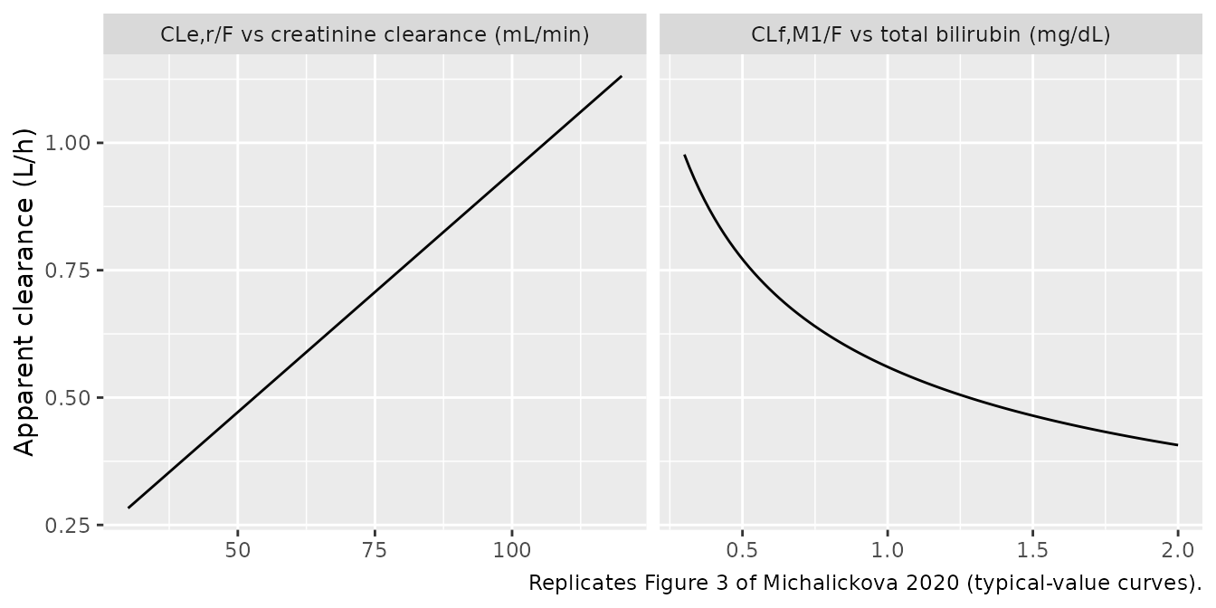
| CLe,r/F = CLe,rTV * (CREACL / 70) | n/a | Table 2; Results (‘increase 0.009 L/h per unit’) |
| CLf,M1/F = CLf,M1TV * (BILTOT / 0.69)^theta | n/a | Table 2; Results |
| One-compartment parent -> one-compartment M1, parallel CLe,r | n/a | Figure 2; Results |
| Lag time only when MIX_LAGGED_ABS = 1 | n/a | Methods ‘Covariate analysis’; Results |
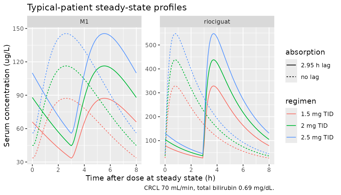
Typical-value steady-state profiles
The patients were at steady state on three-times-daily dosing, so
every simulation below starts from a steady-state dose
(ss = 1, ii = 8). The model has two endpoints
(Cc and Cc_m1) and neither is an ODE state.
Observation rows are therefore keyed by dvid (1 =
riociguat, 2 = M1) with cmt left empty. Typical-value
solves use omega = NA, sigma = NA.
mod <- readModelDb("Michalickova_2020_riociguat")

ref_cov <- tibble(CRCL = 70, TBILI = 0.69 * 17.1) # cohort medians; TBILI in umol/L

make_ss_events <- function(dose_mg, lagged, id, obs_times = seq(0, 8, by = 0.1)) {
  dose <- tibble(
    id = id, time = 0, amt = dose_mg, evid = 1L, cmt = "depot",
    ii = 8, ss = 1L, dvid = NA_integer_
  )
  obs <- tidyr::expand_grid(time = obs_times, dvid = 1:2) |>
    mutate(
      id = id, amt = NA_real_, evid = 0L, cmt = NA_character_,
      ii = 0, ss = 0L
    )
  bind_rows(dose, obs) |>
    mutate(
      MIX_LAGGED_ABS = lagged, dose_mg = dose_mg,
      CRCL = ref_cov$CRCL, TBILI = ref_cov$TBILI
    )
}

scen <- tidyr::expand_grid(dose_mg = c(1.5, 2, 2.5), lagged = c(0, 1)) |>
  mutate(id = seq_len(n()))
ev_typ <- lapply(seq_len(nrow(scen)), function(i) {
  make_ss_events(scen$dose_mg[i], scen$lagged[i], scen$id[i])
}) |>
  bind_rows() |>
  arrange(id, time, desc(evid))

sim_typ <- rxode2::rxSolve(
  mod, ev_typ,
  omega = NA, sigma = NA, useLinCmt = FALSE,
  returnType = "data.frame",
  keep = c("dose_mg", "MIX_LAGGED_ABS"),
  rtol = 1e-10, atol = 1e-12, ssRtol = 1e-10, ssAtol = 1e-12
) |>
  distinct(id, time, .keep_all = TRUE) |>
  mutate(
    regimen = paste0(dose_mg, " mg TID"),
    absorption = ifelse(MIX_LAGGED_ABS == 1, "2.95 h lag", "no lag")
  )
sim_typ |>
  select(time, regimen, absorption, riociguat = Cc, M1 = Cc_m1) |>
  pivot_longer(c(riociguat, M1), names_to = "analyte", values_to = "conc") |>
  ggplot(aes(time, conc, colour = regimen, linetype = absorption)) +
  geom_line() +
  facet_wrap(~analyte, scales = "free_y") +
  labs(
    x = "Time after dose at steady state (h)",
    y = "Serum concentration (ug/L)",
    title = "Typical-patient steady-state profiles",
    caption = "CRCL 70 mL/min, total bilirubin 0.69 mg/dL."
  )
Closed-form check
For a linear model the steady-state average concentration over a
dosing interval follows directly from the clearances. Riociguat averages
Dose / tau / (CLf,M1/F + CLe,r/F). M1 averages
Dose / tau * CLf,M1 / (CLf,M1 + CLe,r) / CLe,M1. The lag
time shifts the profile in time and leaves both averages unchanged.
PKNCA’s cav over one steady-state interval must reproduce
these closed forms. The two sides use identical parameters, so the
tolerance only has to cover numerical integration error.
cl_met <- 0.665
cl_nonmet <- 0.66
cl_m1 <- 1.47
closed_form <- scen |>
  mutate(
    regimen = paste0(dose_mg, " mg TID"),
    absorption = ifelse(lagged == 1, "2.95 h lag", "no lag"),
    cav_parent = dose_mg / 8 / (cl_met + cl_nonmet) * 1000,
    cav_m1 = dose_mg / 8 * cl_met / (cl_met + cl_nonmet) / cl_m1 * 1000
  )

run_nca <- function(sim, conc_col) {
  conc <- sim |>
    filter(!is.na(.data[[conc_col]])) |>
    transmute(id, time, conc = .data[[conc_col]], regimen, absorption)
  dose <- sim |>
    distinct(id, regimen, absorption, dose_mg) |>
    mutate(time = 0)
  o_conc <- PKNCA::PKNCAconc(conc, conc ~ time | regimen + absorption + id)
  o_dose <- PKNCA::PKNCAdose(dose, dose_mg ~ time | regimen + absorption + id)
  intervals <- data.frame(
    start = 0, end = 8, cmax = TRUE, tmax = TRUE, cmin = TRUE,
    auclast = TRUE, cav = TRUE
  )
  res <- PKNCA::pk.nca(PKNCA::PKNCAdata(o_conc, o_dose, intervals = intervals))
  as.data.frame(res)
}

nca_parent <- run_nca(sim_typ, "Cc")
nca_m1 <- run_nca(sim_typ, "Cc_m1")

cav_check <- bind_rows(
  nca_parent |> filter(PPTESTCD == "cav") |> mutate(analyte = "riociguat"),
  nca_m1 |> filter(PPTESTCD == "cav") |> mutate(analyte = "M1")
) |>
  left_join(closed_form, by = c("regimen", "absorption")) |>
  mutate(
    closed = ifelse(analyte == "riociguat", cav_parent, cav_m1),
    rel_err = PPORRES / closed - 1
  )

# PKNCA integrates a 0.1 h grid with the linear-up/log-down trapezoid, so the
# difference is trapezoidal error on the narrow absorption peak (~0.1-0.3%
# measured), not model error. A mis-transcribed clearance or volume unit would
# move these averages by tens of percent.
stopifnot(max(abs(cav_check$rel_err)) < 0.01)

cav_check |>
  select(analyte, regimen, absorption, PPORRES, closed, rel_err) |>
  mutate(rel_err = sprintf("%.3f%%", 100 * rel_err)) |>
  rename(
    "Analyte" = analyte, "Regimen" = regimen, "Absorption" = absorption,
    "Cav simulated (ug/L)" = PPORRES, "Cav closed form (ug/L)" = closed,
    "Relative difference" = rel_err
  ) |>
knitr::kable(digits = 1)| Analyte | Regimen | Absorption | Cav simulated (ug/L) | Cav closed form (ug/L) | Relative difference |
|---|---|---|---|---|---|
| riociguat | 1.5 mg TID | 2.95 h lag | 141.6 | 141.5 | 0.038% |
| riociguat | 1.5 mg TID | no lag | 141.4 | 141.5 | -0.099% |
| riociguat | 2 mg TID | 2.95 h lag | 188.8 | 188.7 | 0.038% |
| riociguat | 2 mg TID | no lag | 188.5 | 188.7 | -0.099% |
| riociguat | 2.5 mg TID | 2.95 h lag | 235.9 | 235.8 | 0.038% |
| riociguat | 2.5 mg TID | no lag | 235.6 | 235.8 | -0.099% |
| M1 | 1.5 mg TID | 2.95 h lag | 64.0 | 64.0 | -0.002% |
| M1 | 1.5 mg TID | no lag | 64.0 | 64.0 | -0.002% |
| M1 | 2 mg TID | 2.95 h lag | 85.4 | 85.4 | -0.002% |
| M1 | 2 mg TID | no lag | 85.4 | 85.4 | -0.002% |
| M1 | 2.5 mg TID | 2.95 h lag | 106.7 | 106.7 | -0.002% |
| M1 | 2.5 mg TID | no lag | 106.7 | 106.7 | -0.002% |
PKNCA steady-state summary
The paper reports no NCA summary. The table shows the model’s
steady-state exposures for the typical patient at the three prescribed
dose levels, without the lag time. Both analytes are side by side, with
the closed-form Cav as the reference column.
nca_ref <- closed_form |>
  filter(lagged == 0) |>
  transmute(regimen, analyte = "riociguat", cav = cav_parent) |>
  bind_rows(
    closed_form |> filter(lagged == 0) |>
      transmute(regimen, analyte = "M1", cav = cav_m1)
  )
nca_sim <- bind_rows(
  nca_parent |> mutate(analyte = "riociguat"),
  nca_m1 |> mutate(analyte = "M1")
) |>
  filter(absorption == "no lag") |>
  select(regimen, analyte, PPTESTCD, PPORRES)

tab <- nlmixr2lib::ncaComparisonTable(
  simulated = nca_sim,
  reference = nca_ref,
  by = c("regimen", "analyte"),
  params = "cav",
  units = c(cav = "ug/L")
)
knitr::kable(tab)| NCA parameter | regimen | analyte | Reference | Simulated | % diff |
|---|---|---|---|---|---|
| Cavg (ug/L) | 1.5 mg TID | riociguat | 142 | 141 | -0.1% |
| Cavg (ug/L) | 1.5 mg TID | M1 | 64 | 64 | -0.0% |
| Cavg (ug/L) | 2 mg TID | riociguat | 189 | 188 | -0.1% |
| Cavg (ug/L) | 2 mg TID | M1 | 85.4 | 85.4 | -0.0% |
| Cavg (ug/L) | 2.5 mg TID | riociguat | 236 | 236 | -0.1% |
| Cavg (ug/L) | 2.5 mg TID | M1 | 107 | 107 | -0.0% |
nca_sim |>
  filter(PPTESTCD %in% c("cmax", "tmax", "cmin")) |>
  pivot_wider(names_from = PPTESTCD, values_from = PPORRES) |>
  rename(
    "Regimen" = regimen, "Analyte" = analyte, "Cmax,ss (ug/L)" = cmax,
    "Tmax (h)" = tmax, "Cmin,ss (ug/L)" = cmin
  ) |>
knitr::kable(digits = 2)| Regimen | Analyte | Cmax,ss (ug/L) | Cmin,ss (ug/L) | Tmax (h) |
|---|---|---|---|---|
| 1.5 mg TID | riociguat | 328.67 | 26.82 | 0.8 |
| 2 mg TID | riociguat | 438.23 | 35.76 | 0.8 |
| 2.5 mg TID | riociguat | 547.79 | 44.70 | 0.8 |
| 1.5 mg TID | M1 | 87.26 | 33.66 | 2.6 |
| 2 mg TID | M1 | 116.35 | 44.88 | 2.6 |
| 2.5 mg TID | M1 | 145.43 | 56.10 | 2.6 |
Covariate relationships (Figure 3)
# Replicates Figure 3 of Michalickova 2020: typical CLf,M1/F versus total
# bilirubin and CLe,r/F versus creatinine clearance.
bili <- tibble(tbili_mgdl = seq(0.3, 2.0, length.out = 100)) |>
  mutate(value = 0.665 * (tbili_mgdl / 0.69)^-0.462, panel = "CLf,M1/F vs total bilirubin (mg/dL)", x = tbili_mgdl)
crcl <- tibble(CRCL = seq(30, 120, length.out = 100)) |>
  mutate(value = 0.66 * (CRCL / 70), panel = "CLe,r/F vs creatinine clearance (mL/min)", x = CRCL)
bind_rows(bili, crcl) |>
  ggplot(aes(x, value)) +
  geom_line() +
  facet_wrap(~panel, scales = "free_x") +
  labs(
    x = NULL, y = "Apparent clearance (L/h)",
    caption = "Replicates Figure 3 of Michalickova 2020 (typical-value curves)."
  )
# The printed covariate equations must pass through the Table 2 typical
# values at the reference covariates and reproduce the Results slope.
stopifnot(
  abs(0.66 * (70 / 70) - 0.66) < 1e-12,
  abs(0.665 * (0.69 / 0.69)^-0.462 - 0.665) < 1e-12,
  abs(0.66 / 70 - 0.009) < 0.0005 # Results: '0.009 L/h per unit (mL/min)'
)
Virtual cohort and Figure 1
Figure 1 of the paper plots the single observed riociguat and M1
concentration of each patient against the time since the last dose. The
virtual cohort draws 200 patients. Creatinine clearance and total
bilirubin are log-normal with the Table 1 medians and a spread matched
to the IQRs. Doses are 2.5 mg TID for 70% of patients, 2 mg for 20% and
1.5 mg for 10%, which matches the Table 1 median and IQR. Each patient
has one sampling time drawn uniformly over the observed 1.25-6.75 h
window. MIX_LAGGED_ABS is Bernoulli(6/49). With one sample
per patient the paper could not separate inter-individual from residual
variability, so the proportional error terms carry all of it and the
sim column is the full predictive distribution.
set.seed(20200101)
n_sub <- 200
cohort <- tibble(
  id = seq_len(n_sub),
  # IQR of a log-normal = median * exp(+/- 0.674 sigma)
  CRCL = 70 * exp(rnorm(n_sub, 0, log(79 / 59) / (2 * 0.674))),
  tbili_mgdl = 0.69 * exp(rnorm(n_sub, 0, log(0.98 / 0.53) / (2 * 0.674))),
  dose_mg = sample(c(2.5, 2, 1.5), n_sub, replace = TRUE, prob = c(0.7, 0.2, 0.1)),
  MIX_LAGGED_ABS = rbinom(n_sub, 1, 6 / 49),
  tobs = runif(n_sub, 1.25, 6.75)
) |>
  mutate(TBILI = tbili_mgdl * 17.1)

ev_cohort <- bind_rows(
  cohort |> transmute(
    id, time = 0, amt = dose_mg, evid = 1L, cmt = "depot", ii = 8, ss = 1L,
    dvid = NA_integer_, CRCL, TBILI, MIX_LAGGED_ABS
  ),
  tidyr::expand_grid(cohort, dvid = 1:2) |> transmute(
    id, time = tobs, amt = NA_real_, evid = 0L, cmt = NA_character_, ii = 0,
    ss = 0L, dvid, CRCL, TBILI, MIX_LAGGED_ABS
  )
) |>
  arrange(id, time, desc(evid), dvid)

sim_vpc <- suppressWarnings(rxode2::rxSolve(
  mod, ev_cohort,
  useLinCmt = FALSE, returnType = "data.frame",
  keep = c("MIX_LAGGED_ABS")
)) |>
  group_by(id) |>
  mutate(analyte = c("riociguat", "M1")[row_number()]) |>
  ungroup()

# Each subject has exactly two observation rows (dvid 1 then 2). Confirm the
# row-to-endpoint mapping from the output itself: on the riociguat row the
# residual-free prediction ipredSim equals Cc, on the M1 row it equals Cc_m1.
stopifnot(
  all(count(sim_vpc, id)$n == 2),
  with(filter(sim_vpc, analyte == "riociguat"), all(abs(ipredSim / Cc - 1) < 1e-8)),
  with(filter(sim_vpc, analyte == "M1"), all(abs(ipredSim / Cc_m1 - 1) < 1e-8))
)
# Replicates Figure 1 of Michalickova 2020 with simulated observations.
observed_range <- tibble(
  analyte = c("riociguat", "M1"), lo = c(44, 17), hi = c(749, 314)
)
sim_vpc |>
  mutate(absorption = ifelse(MIX_LAGGED_ABS == 1, "2.95 h lag", "no lag")) |>
  ggplot(aes(time, sim)) +
  geom_rect(
    data = observed_range, inherit.aes = FALSE,
    aes(xmin = 1.25, xmax = 6.75, ymin = lo, ymax = hi),
    fill = "grey85", alpha = 0.6
  ) +
  geom_point(aes(shape = absorption), alpha = 0.7) +
  facet_wrap(~analyte, ncol = 1, scales = "free_y") +
  labs(
    x = "Time after the last dose (h)", y = "Serum concentration (ug/L)",
    shape = NULL,
    caption = paste(
      "Simulated single steady-state samples (n = 200). Grey box: observed",
      "time window and concentration range reported by Michalickova 2020."
    )
  )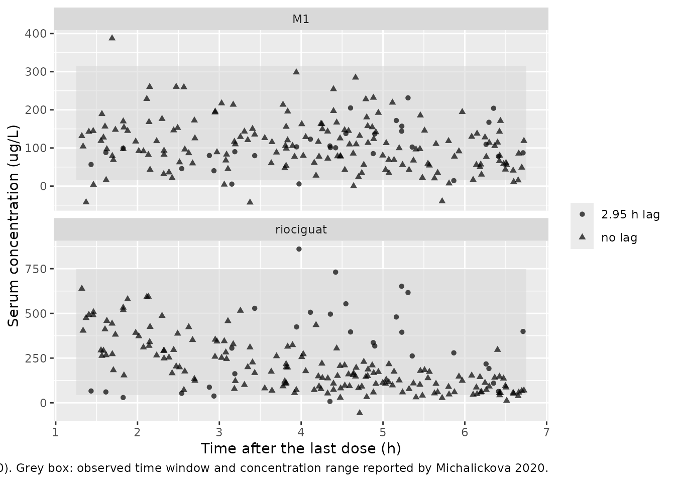
The published figure shows riociguat mostly between about 60 and 600 ug/L and M1 between about 20 and 300 ug/L. The simulated cloud occupies the same region. The check below is on the centre and on robust quantiles of the simulated distribution, not on its extremes (see the repository notes on cohort assertions). It confirms that most simulated samples fall inside the observed range and that the simulated medians match the observed data.
vpc_summary <- sim_vpc |>
  left_join(observed_range, by = "analyte") |>
  group_by(analyte) |>
  summarise(
    median_sim = median(sim),
    q10 = quantile(sim, 0.10), q90 = quantile(sim, 0.90),
    frac_in_observed_range = mean(sim >= lo & sim <= hi),
    .groups = "drop"
  )
knitr::kable(vpc_summary, digits = 2)| analyte | median_sim | q10 | q90 | frac_in_observed_range |
|---|---|---|---|---|
| M1 | 102.65 | 31.26 | 194.47 | 0.92 |
| riociguat | 167.03 | 54.91 | 475.10 | 0.94 |
# Observed medians read from Figure 1 are about 200 ug/L (riociguat) and
# 110 ug/L (M1). A factor-of-two band leaves room for the 200-subject sampling
# noise (the median's MC-SE is ~5%) and still fails on a unit or
# volume transcription error, which moves concentrations by 10x or more.
stopifnot(
  all(vpc_summary$frac_in_observed_range > 0.75),
  with(vpc_summary, median_sim[analyte == "riociguat"] > 100 &
    median_sim[analyte == "riociguat"] < 400),
  with(vpc_summary, median_sim[analyte == "M1"] > 55 &
    median_sim[analyte == "M1"] < 220)
)
Assumptions and deviations
-
Inter-individual variability. With one sample per
patient the authors could not separate inter-individual from residual
variability (Methods). The model therefore has no etas and the Table 2
proportional variances (0.152 and 0.268) cover both. They are encoded as
SDs (
sqrt(variance)). Individual predictions (Cc,Cc_m1) are typical values for the given covariates. Use thesimcolumn for the predictive distribution. -
Lag-time subgroup. The 2.95 h lag applies only to
the six patients whose concentrations were unexpectedly high late after
the dose. It is encoded with the binary covariate
MIX_LAGGED_ABS. The paper suggests food as a possible cause but cannot confirm it. Set it to 0 for a typical patient. -
Covariate units. Total bilirubin enters as the
canonical
TBILIcolumn in umol/L. The model converts it to the paper’s mg/dL with a factor of 17.1. Creatinine clearance (CRCL) is used in mL/min as reported. The paper calls it a CKD-EPI estimate but does not say whether it was de-normalised from mL/min/1.73 m^2. - Bilirubin exponent. Table 2 gives -0.462 and the Results text -0.463. The Table 2 final-model value is used.
- Metabolite mass balance. The paper does not mention a molecular-weight correction for the conversion of riociguat (MW 422.4) to M1 (MW 408.4), so M1 is formed 1:1 on a mass basis. Correcting for it would lower M1 concentrations by about 3%. The M1 parameters depend on the assumption that the two volumes are equal (Discussion), so absolute M1 parameter values should be read with that in mind.
- ka. Fixed at 3 1/h from Saleh 2016 (single-dose riociguat popPK). The paper labels it ‘Ka/F’, but a rate constant is not scaled by bioavailability, so it is treated as ka.
- Virtual-cohort covariates. Log-normal distributions matched to the Table 1 medians and IQRs, independent of each other. The dose mix is an assumption consistent with the Table 1 median and IQR.
- Errata. No erratum or correction was found for this article (literature check on 2026-09-25).