Busulfan and sulfolane (Dadkhah 2022)
Source:vignettes/articles/Dadkhah_2022_busulfan.Rmd
Dadkhah_2022_busulfan.RmdModel and source
- Citation: Dadkhah A, Wicha SG, Kroger N, Muller A, Pfaffendorf C, Riedner M, Badbaran A, Fehse B, Langebrake C. Population Pharmacokinetics of Busulfan and Its Metabolite Sulfolane in Patients with Myelofibrosis Undergoing Hematopoietic Stem Cell Transplantation. Pharmaceutics. 2022;14(6):1145. doi:10.3390/pharmaceutics14061145. Structure from Figure 1; covariate equations (1) and (2) from Section 3.3; parameter estimates from Table 2.
- Description: Joint parent-metabolite population PK model for intravenous busulfan and its metabolite sulfolane in adults with myelofibrosis receiving reduced-intensity busulfan/fludarabine conditioning before allogeneic haematopoietic stem cell transplantation (Dadkhah 2022). One compartment for each analyte with first-order elimination; a fixed metabolic fraction (MF = 0.0704) of total busulfan clearance forms sulfolane. Total body weight enters busulfan volume as a power function (exponent 0.854, 75 kg reference) and the GSTA1 -52G>A (rs3957356) SNP multiplies sulfolane clearance by exp(1.43). Log-normal IIV on all four clearances and volumes, inter-occasion variability on busulfan clearance (one occasion per sampled administration, up to three), and a proportional residual error per analyte.
- Article: https://doi.org/10.3390/pharmaceutics14061145 (open access)
Dadkhah 2022 fitted busulfan and its metabolite sulfolane together in adults with myelofibrosis who received reduced-intensity busulfan/fludarabine conditioning before allogeneic stem cell transplantation. Each analyte has one compartment. A fixed fraction (MF = 7.04%) of total busulfan clearance forms sulfolane (Figure 1). Total body weight scales busulfan volume, and a GSTA1 promoter SNP (-52G>A, rs3957356) raises sulfolane clearance. Busulfan clearance carries inter-occasion variability.
Population
Thirty-seven patients with myelofibrosis (19 female, 18 male) were treated at the University Medical Center Hamburg-Eppendorf. Thirty were enrolled prospectively between November 2018 and June 2020 and seven retrospectively from October 2016 to October 2017 (Section 2.1 and Section 3.1). Median age was 60 years (IQR 53.5-65.5) and median total body weight 75 kg (IQR 64.05-88.25) (Table 1). Eighteen patients had primary myelofibrosis, 9 post-essential thrombocythaemia and 10 post-polycythaemia vera myelofibrosis. The GSTA1 -52G>A SNP was found in 28 patients (75.7%) and a GSTM1 deletion in 19.
Thirty patients (81%) received ten 0.8 mg/kg doses of busulfan, each a 2 h infusion every 6 h (Q6H). Seven (19%) received three 3.2 mg/kg doses as 3 h infusions every 24 h (Q24H), with the later doses adjusted where needed to a cumulative AUC (cAUC) of 50 mg x h/L (Section 2.2). The dataset held 282 busulfan and 241 sulfolane concentrations. Sulfolane was measured only in the prospective patients, and 70 sulfolane samples were below the 0.04 mg/L limit of quantification.
The same information is available programmatically:
pop <- rxode2::rxode(readModelDb("Dadkhah_2022_busulfan"))$population
#> ℹ parameter labels from comments will be replaced by 'label()'
#> Warning: some etas defaulted to non-mu referenced, possible parsing error: etaiov_cl_1, etaiov_cl_2, etaiov_cl_3
#> as a work-around try putting the mu-referenced expression on a simple line
str(pop, max.level = 1)
#> List of 16
#>  $ species         : chr "human"
#>  $ n_subjects      : int 37
#>  $ n_studies       : int 1
#>  $ age_range       : chr "median 60 years (IQR 53.5-65.5); adults >= 18 years"
#>  $ weight_range    : chr "median 75 kg (IQR 64.05-88.25)"
#>  $ height          : chr "median 174 cm (IQR 168-181)"
#>  $ bsa             : chr "median 1.84 m^2 (IQR 1.75-2.07)"
#>  $ sex_female_pct  : num 51.4
#>  $ race_ethnicity  : chr "Not reported."
#>  $ disease_state   : chr "Myelofibrosis scheduled for allogeneic haematopoietic stem cell transplantation after reduced-intensity busulfa"| __truncated__
#>  $ dose_range      : chr "Q6H regimen (30 patients, 81%): 10 doses of 0.8 mg/kg intravenous busulfan every 6 h, each a 2 h infusion. Q24H"| __truncated__
#>  $ genotype        : chr "GSTA1 -52G>A (rs3957356) SNP 28 (75.7%); GSTM1 deletion 19 (51.35%); both 10 (27%)."
#>  $ hepatic_function: chr "AST median 21 U/L, ALT median 21 U/L, alkaline phosphatase median 85 U/L, bilirubin median 0.6 mg/dL, albumin m"| __truncated__
#>  $ regions         : chr "Germany (University Medical Center Hamburg-Eppendorf; prospective November 2018 - June 2020 plus retrospective "| __truncated__
#>  $ n_observations  : chr "523 plasma concentrations: 282 busulfan and 241 sulfolane. Sulfolane was measured only in the 30 prospectively "| __truncated__
#>  $ notes           : chr "Demographics from Table 1 and Section 3.1. NONMEM 7.4.3, FOCE-I; parameter uncertainty from SIR (M/m = 5000/1000)."
Source trace
Each ini() entry in
inst/modeldb/specificDrugs/Dadkhah_2022_busulfan.R carries
its source as an in-file comment. The table below collects them.
| Equation / parameter | Value | Source location |
|---|---|---|
| Structure | 1-cmt busulfan, 1-cmt sulfolane, IV infusion | Section 3.2; Figure 1 |
Formation fm * kel * central
|
sulfolane formed from total CLBu | Figure 1 arrow ‘CLBu x MF’ and caption |
lcl (CLBu) |
16.3 L/h | Table 2 (RSE 3.6%); Section 3.3 |
lvc (VBu, 75 kg) |
61.5 L | Table 2 (RSE 2%) |
e_wt_vc |
0.854 | Table 2 ’COV_V Bu _TBW’; equation (1)
VBu = VBu-typ * (TBW/75)^0.854
|
fm (MF) |
0.0704 | Table 2 (RSE 28.6%) |
lcl_sulfolane (CLSu, non-carrier) |
1.61 L/h | Table 2 (RSE 37%) |
lvc_sulfolane (VSu) |
48.8 L | Table 2 (RSE 35.2%) |
e_gsta1_cl_sulfolane |
1.43 | Table 2 ’COV_CL Su _GSTA1’; equation (2)
CLSu = CLSu-typ * e^1.43 for GSTA1 |
etalcl |
0.045171 | Table 2 ‘IIV CL Bu’ 21.5% CV; log(1 + CV^2) per the
Table 2 footnote |
etalvc |
0.009950 | Table 2 ‘IIV V Bu’ 10% CV |
etalcl_sulfolane |
0.820843 | Table 2 ‘IIV CL Su’ 112.8% CV |
etalvc_sulfolane |
0.471361 | Table 2 ‘IIV V Su’ 77.6% CV |
etaiov_cl_1..3 |
0.005759 each | Table 2 ‘IOV CL Bu’ 7.6% CV; occasions defined in Section 3.2 |
propSd |
0.071 | Table 2 ‘Prop. sigma Bu’ 7.1% |
propSd_sulfolane |
0.362 | Table 2 ‘Prop. sigma Su’ 36.2% |
Typical values against the abstract
The abstract quotes the typical parameters per kilogram for a 75 kg patient: busulfan CL 0.217 L/h/kg and V 0.82 L/kg, sulfolane CL 0.021 L/h/kg and V 0.65 L/kg. These come from the same Table 2 estimates, so only rounding separates them.
mod <- readModelDb("Dadkhah_2022_busulfan")

ev_typ <- data.frame(
  id = 1L, time = 0, evid = 0L, amt = 0, cmt = "central", dvid = 1L,
  WT = 75, SNP_GSTA1_RS3957356 = 0L, OCC = 1L
)
typ <- rxode2::rxSolve(rxode2::zeroRe(mod), events = ev_typ, useLinCmt = FALSE) |>
  as.data.frame()
#> ℹ parameter labels from comments will be replaced by 'label()'
#> Warning: some etas defaulted to non-mu referenced, possible parsing error: etaiov_cl_1, etaiov_cl_2, etaiov_cl_3
#> as a work-around try putting the mu-referenced expression on a simple line
#> Warning: some etas defaulted to non-mu referenced, possible parsing error: etaiov_cl_1, etaiov_cl_2, etaiov_cl_3
#> as a work-around try putting the mu-referenced expression on a simple line
#> ℹ omega/sigma items treated as zero: 'etalcl', 'etalvc', 'etalcl_sulfolane', 'etalvc_sulfolane', 'etaiov_cl_1', 'etaiov_cl_2', 'etaiov_cl_3'

typ_tab <- tibble::tibble(
  parameter = c("Busulfan CL (L/h/kg)", "Busulfan V (L/kg)", "Sulfolane CL (L/h/kg)", "Sulfolane V (L/kg)"),
  model = c(typ$cl, typ$vc, typ$cl_sulfolane, typ$vc_sulfolane) / 75,
  abstract = c(0.217, 0.82, 0.021, 0.65)
)
typ_tab |>
  dplyr::rename("Parameter" = parameter, "Model" = model, "Abstract" = abstract) |>
knitr::kable(digits = 4, caption = "Typical values for a 75 kg GSTA1 SNP non-carrier.")| Parameter | Model | Abstract |
|---|---|---|
| Busulfan CL (L/h/kg) | 0.2173 | 0.217 |
| Busulfan V (L/kg) | 0.8200 | 0.820 |
| Sulfolane CL (L/h/kg) | 0.0215 | 0.021 |
| Sulfolane V (L/kg) | 0.6507 | 0.650 |
Virtual cohort
The individual data are not public. Body weight is drawn log-normally
with the Table 1 median (75 kg) and a spread matching its interquartile
range (64.05-88.25 kg, so
sdlog = log(88.25 / 64.05) / 1.349 = 0.238), truncated to
40-150 kg. Each subject carries the GSTA1 SNP with probability
0.757.
Occasions follow Section 3.2: each sampled administration opens a new occasion. Q6H patients were sampled after the first, fifth and ninth infusions, so doses 1-4 are occasion 1, doses 5-8 occasion 2 and doses 9-10 occasion 3. Q24H patients were sampled after the first infusion only, so all three of their doses are occasion 1.
set.seed(20220527)
rxode2::rxSetSeed(20220527)

n_q6h <- 200L
n_q24h <- 200L

draw_wt <- function(n) {
  wt <- exp(rnorm(n, log(75), log(88.25 / 64.05) / 1.349))
  pmin(pmax(wt, 40), 150)
}

subj_q6h <- tibble::tibble(
  id = seq_len(n_q6h),
  regimen = "Q6H",
  WT = draw_wt(n_q6h),
  SNP_GSTA1_RS3957356 = rbinom(n_q6h, 1, 0.757)
)
subj_q24h <- tibble::tibble(
  id = n_q6h + seq_len(n_q24h),
  regimen = "Q24H",
  WT = draw_wt(n_q24h),
  SNP_GSTA1_RS3957356 = rbinom(n_q24h, 1, 0.757)
)

# Observation rows sit on the busulfan state with dvid = 1; rxode2 returns
# both Cc and Cc_sulfolane as columns at every observation time.
make_events <- function(subj, dose_times, dose_mgkg, inf_dur, obs_times, occ_breaks) {
  doses <- tidyr::crossing(subj, time = dose_times) |>
    dplyr::mutate(evid = 1L, amt = dose_mgkg * WT, rate = amt / inf_dur, dvid = NA_integer_)
  obs <- tidyr::crossing(subj, time = obs_times) |>
    dplyr::mutate(evid = 0L, amt = 0, rate = 0, dvid = 1L)
  dplyr::bind_rows(doses, obs) |>
    dplyr::mutate(
      cmt = "central",
      OCC = findInterval(time, occ_breaks)
    ) |>
    dplyr::arrange(id, time, dplyr::desc(evid)) |>
    as.data.frame()
}

grid_q6h <- sort(unique(c(seq(0, 84, by = 0.25), 2.08, 48 + 2.08)))
ev_q6h <- make_events(
  subj_q6h,
  dose_times = seq(0, 54, by = 6), dose_mgkg = 0.8, inf_dur = 2,
  obs_times = grid_q6h, occ_breaks = c(0, 24, 48)
)
# Q24H: first dose only (the later doses depend on the TDM result, below).
ev_q24h <- make_events(
  subj_q24h,
  dose_times = 0, dose_mgkg = 3.2, inf_dur = 3,
  obs_times = seq(0, 36, by = 0.25), occ_breaks = 0
)
stopifnot(
  !anyDuplicated(ev_q6h[, c("id", "time", "evid")]),
  setequal(unique(ev_q6h$OCC), 1:3),
  all(ev_q24h$OCC == 1L)
)
summary(subj_q6h$WT)
#>    Min. 1st Qu.  Median    Mean 3rd Qu.    Max.
#>   40.00   66.16   75.93   78.08   87.75  134.55
Simulation
sim_q6h <- rxode2::rxSolve(
  mod,
  events = ev_q6h, keep = c("regimen", "WT", "SNP_GSTA1_RS3957356"), useLinCmt = FALSE
) |>
  as.data.frame()
#> ℹ parameter labels from comments will be replaced by 'label()'
#> Warning: some etas defaulted to non-mu referenced, possible parsing error: etaiov_cl_1, etaiov_cl_2, etaiov_cl_3
#> as a work-around try putting the mu-referenced expression on a simple line
sim_q24h <- rxode2::rxSolve(
  mod,
  events = ev_q24h, keep = c("regimen", "WT", "SNP_GSTA1_RS3957356"), useLinCmt = FALSE
) |>
  as.data.frame()
stopifnot(!anyNA(sim_q6h$Cc), !anyNA(sim_q6h$Cc_sulfolane), !anyNA(sim_q24h$Cc))
Replicate published results
Concentration-time profiles (Figure 3)
Figure 3 of the paper is a prediction-corrected VPC for the Q6H patients, plotted against time after the first and ninth doses. The panels below show the 5th, 50th and 95th percentiles of the simulated Q6H concentrations, including residual error, over the whole 10-dose course. The grey line in the sulfolane panel marks the 0.04 mg/L LLOQ. Residual error is added to each analyte by hand because the observation rows carry the busulfan endpoint.
vpc <- sim_q6h |>
  dplyr::mutate(
    Busulfan = Cc * (1 + 0.071 * rnorm(dplyr::n())),
    Sulfolane = Cc_sulfolane * (1 + 0.362 * rnorm(dplyr::n()))
  ) |>
  dplyr::select(id, time, Busulfan, Sulfolane) |>
  tidyr::pivot_longer(c(Busulfan, Sulfolane), names_to = "analyte", values_to = "conc") |>
  dplyr::group_by(analyte, time) |>
  dplyr::summarise(
    Q05 = quantile(conc, 0.05), Q50 = quantile(conc, 0.50), Q95 = quantile(conc, 0.95),
    .groups = "drop"
  )

ggplot(vpc, aes(time, Q50)) +
  geom_ribbon(aes(ymin = Q05, ymax = Q95), alpha = 0.25) +
  geom_line() +
  geom_hline(
    data = data.frame(analyte = "Sulfolane", y = 0.04), aes(yintercept = y),
    colour = "grey50"
  ) +
  facet_wrap(~analyte, scales = "free_y", ncol = 1) +
  labs(
    x = "Time since first dose (h)",
    y = "Concentration (mg/L)",
    caption = "Simulated Q6H 5th-50th-95th percentiles; compare with Figure 3 of Dadkhah 2022."
  )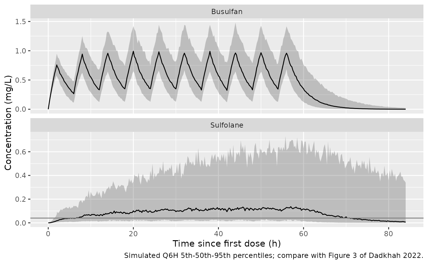
Sulfolane accumulates over the course because its typical half-life
(log(2) * 48.8 / 1.61 = 21 h in non-carriers, 5 h in
carriers) is long against the 6 h dosing interval.
Sulfolane below the limit of quantification
Section 3.1 reports 70 of 241 sulfolane samples (29%) below 0.04 mg/L. Here the simulated Q6H concentrations, with residual error, are read at the protocol sampling times: 2.08, 3, 4 and 5.5 h after the first and ninth infusions and 5.5 h after the fifth (Section 2.2).
samp_times <- c(2.08, 3, 4, 5.5, 24 + 5.5, 48 + c(2.08, 3, 4, 5.5))
blq <- sim_q6h |>
  dplyr::filter(time %in% samp_times) |>
  dplyr::mutate(obs = Cc_sulfolane * (1 + 0.362 * rnorm(dplyr::n())), blq = obs < 0.04)

blq_by_time <- blq |>
  dplyr::group_by(time) |>
  dplyr::summarise(pct_blq = 100 * mean(blq), .groups = "drop")
blq_by_time |>
  dplyr::rename("Time since first dose (h)" = time, "Simulated BLQ (%)" = pct_blq) |>
knitr::kable(digits = 1, caption = "Share of simulated sulfolane samples below 0.04 mg/L.")| Time since first dose (h) | Simulated BLQ (%) |
|---|---|
| 2.1 | 83.5 |
| 3.0 | 67.0 |
| 4.0 | 53.0 |
| 5.5 | 52.0 |
| 29.5 | 19.5 |
| 50.1 | 16.5 |
| 51.0 | 12.5 |
| 52.0 | 15.0 |
| 53.5 | 17.0 |
overall_blq <- 100 * mean(blq$blq)
overall_blq
#> [1] 37.33333
Overall 37% of the simulated samples are below the LLOQ, against 29% observed. Most come from the first dosing day, before sulfolane has accumulated, as in the lower panel of Figure 3B. The observed share also includes the Q24H patients’ samples, and the paper does not give the sample count per time point, so this check is reported but not gated.
Busulfan cumulative AUC (Section 3.1)
Section 3.1 reports a median busulfan cAUC of 36.06 mg x h/L (range 25.67-61.85) over all 37 patients. PKNCA computes the Q6H cAUC from the dense simulated profile from 0 to 84 h (30 h after the last infusion). For the Q24H arm, PKNCA computes the first-dose AUC to infinity, and the second and third doses are then set so that the cAUC reaches 50 mg x h/L (Section 2.2). Because Q24H patients have a single occasion and the model is linear, the adjusted cAUC is exactly 50 by construction.
nca_conc <- dplyr::bind_rows(sim_q6h, sim_q24h) |>
  dplyr::filter(!is.na(Cc)) |>
  dplyr::select(id, regimen, time, Cc)
nca_dose <- dplyr::bind_rows(ev_q6h, ev_q24h) |>
  dplyr::filter(evid == 1L) |>
  dplyr::select(id, regimen, time, amt)

conc_obj <- PKNCA::PKNCAconc(nca_conc, Cc ~ time | regimen + id)
dose_obj <- PKNCA::PKNCAdose(nca_dose, amt ~ time | regimen + id)
# Q6H: the whole course (cAUC), the three occasion windows, and the first
# dosing interval. Q24H: first dose to infinity and its first 24 h.
intervals <- data.frame(
  regimen = c("Q6H", "Q6H", "Q6H", "Q6H", "Q6H", "Q24H", "Q24H"),
  start = c(0, 0, 24, 48, 0, 0, 0),
  end = c(84, 24, 48, 84, 6, Inf, 24),
  auclast = c(TRUE, TRUE, TRUE, TRUE, FALSE, FALSE, FALSE),
  aucinf.obs = c(FALSE, FALSE, FALSE, FALSE, FALSE, TRUE, FALSE),
  cmax = c(FALSE, FALSE, FALSE, FALSE, TRUE, FALSE, TRUE),
  tmax = c(FALSE, FALSE, FALSE, FALSE, TRUE, FALSE, TRUE)
)
nca_res <- PKNCA::pk.nca(PKNCA::PKNCAdata(
  conc_obj, dose_obj,
  intervals = intervals,
  options = list(auc.method = "lin up/log down")
))
nca_df <- as.data.frame(nca_res)
summary(nca_res)
#>  start end regimen   N     auclast         cmax              tmax  aucinf.obs
#>      0  84     Q6H 200 37.6 [34.4]            .                 .           .
#>      0  24     Q6H 200 13.6 [29.6]            .                 .           .
#>     24  48     Q6H 200 15.0 [34.9]            .                 .           .
#>     48  84     Q6H 200 8.93 [42.8]            .                 .           .
#>      0   6     Q6H 200           . 0.754 [13.8] 2.00 [2.00, 2.00]           .
#>      0 Inf    Q24H 200           .            .                 . 14.6 [32.2]
#>      0  24    Q24H 200           .  2.61 [14.9] 3.00 [3.00, 3.00]           .
#>
#> Caption: auclast, cmax, aucinf.obs: geometric mean and geometric coefficient of variation; tmax: median and range; N: number of subjects
The PKNCA AUCs are checked against mass balance. Busulfan is
eliminated only through CL, so over the whole course the total dose
equals sum(CL_k * AUC_k), where AUC_k is the
AUC within occasion k’s time window and CL_k is that
occasion’s clearance. (A simpler sum(dose / CL) is not
exact here: drug still in the body when a new occasion opens is cleared
at the new occasion’s clearance.) The busulfan still in the body at 84 h
is added to the eliminated amount, since heavy subjects with low
clearance have a half-life of several hours. The two sides share the
drawn parameters, so only the trapezoidal error separates them.
cl_occ <- sim_q6h |>
  dplyr::distinct(id, OCC, cl)
q6h_auc <- nca_df |>
  dplyr::filter(regimen == "Q6H", PPTESTCD == "auclast")
mass_balance <- q6h_auc |>
  dplyr::filter(end != 84 | start != 0) |>
  dplyr::mutate(OCC = findInterval(start, c(0, 24, 48))) |>
  dplyr::left_join(cl_occ, by = c("id", "OCC")) |>
  dplyr::group_by(id) |>
  dplyr::summarise(eliminated = sum(cl * PPORRES), .groups = "drop") |>
  dplyr::left_join(
    sim_q6h |>
      dplyr::filter(time == 84) |>
      dplyr::select(id, remaining = central),
    by = "id"
  ) |>
  dplyr::left_join(
    ev_q6h |>
      dplyr::filter(evid == 1L) |>
      dplyr::group_by(id) |>
      dplyr::summarise(total_dose = sum(amt), .groups = "drop"),
    by = "id"
  )

cauc_q6h <- q6h_auc |>
  dplyr::filter(start == 0, end == 84) |>
  dplyr::select(id, cauc = PPORRES)
stopifnot(
  nrow(cauc_q6h) == n_q6h,
  nrow(mass_balance) == n_q6h,
  max(abs((mass_balance$eliminated + mass_balance$remaining) / mass_balance$total_dose - 1)) < 0.01
)

auc1_q24h <- nca_df |>
  dplyr::filter(regimen == "Q24H", PPTESTCD == "aucinf.obs") |>
  dplyr::select(id, auc1 = PPORRES) |>
  dplyr::left_join(dplyr::distinct(sim_q24h, id, cl), by = "id") |>
  dplyr::left_join(dplyr::select(subj_q24h, id, WT), by = "id")
stopifnot(max(abs(auc1_q24h$auc1 / (3.2 * auc1_q24h$WT / auc1_q24h$cl) - 1)) < 0.01)

# Doses 2 and 3 share the remaining exposure: (50 - AUC1) * CL each half.
q24h_adj <- auc1_q24h |>
  dplyr::mutate(
    dose23_mgkg = (50 - auc1) * cl / 2 / WT,
    cauc = auc1 + 2 * dose23_mgkg * WT / cl
  )
summary(q24h_adj$dose23_mgkg)
#>    Min. 1st Qu.  Median    Mean 3rd Qu.    Max.
#>  0.7019  2.8260  3.8746  4.1624  5.1460 11.3281
The adjusted Q24H doses (median 3.87 mg/kg) sit a little above the 3.2 mg/kg starting dose, as expected for a 50 mg x h/L target.
The published median covers all 37 patients, 30 of them on Q6H. The table gives the simulated Q6H arm and, for reference, the two arms pooled in the study’s 30:7 ratio (all 200 Q6H subjects plus the first 47 Q24H subjects).
cauc_pool <- c(cauc_q6h$cauc, head(q24h_adj$cauc, round(n_q6h * 7 / 30)))
cauc_tab <- tibble::tibble(
  statistic = c("Median", "Minimum", "Maximum"),
  q6h = c(median(cauc_q6h$cauc), min(cauc_q6h$cauc), max(cauc_q6h$cauc)),
  pooled = c(median(cauc_pool), min(cauc_pool), max(cauc_pool)),
  published = c(36.06, 25.67, 61.85)
)
cauc_tab |>
  dplyr::rename(
    "cAUC (mg*h/L)" = statistic, "Simulated Q6H" = q6h,
    "Simulated Q6H + Q24H (30:7)" = pooled, "Published, all 37 (Section 3.1)" = published
  ) |>
knitr::kable(digits = 2, caption = "Busulfan cumulative AUC.")| cAUC (mg*h/L) | Simulated Q6H | Simulated Q6H + Q24H (30:7) | Published, all 37 (Section 3.1) |
|---|---|---|---|
| Median | 38.07 | 42.20 | 36.06 |
| Minimum | 14.17 | 14.17 | 25.67 |
| Maximum | 93.39 | 93.39 | 61.85 |
# Centre of the Q6H distribution: a mis-transcribed CL, dose or unit would
# move the median by tens of percent.
stopifnot(abs(median(cauc_q6h$cauc) / 36.06 - 1) < 0.1)
The simulated Q6H median is within 6% of the published median. The pooled median runs higher, for two reasons. The simulated Q24H subjects all reach exactly 50 mg x h/L, because their doses are adjusted using their true clearance. The simulated spread is also wider than the observed one: cAUC scales with weight / CL, the model has no weight effect on busulfan clearance, and so the weight spread and the 21.5% CV IIV on clearance add up. The 37 patients span 25.7-61.9 mg x h/L, a 2.4-fold range, while 200 simulated subjects span 6.6-fold. Neither the pooled median nor the range is gated.
Individual busulfan clearance after the first and ninth doses
Section 3.1 gives the median individual busulfan clearance as 17.16 L/h after the first dose (range 10.55-22.36) and 16.47 L/h after the ninth (range 10.05-19.27), from the post hoc estimates. The simulated Q6H clearances on occasions 1 and 3 are summarised below.
cl_tab <- cl_occ |>
  dplyr::filter(OCC %in% c(1L, 3L)) |>
  dplyr::group_by(OCC) |>
  dplyr::summarise(
    median = median(cl), q05 = quantile(cl, 0.05), q95 = quantile(cl, 0.95),
    .groups = "drop"
  ) |>
  dplyr::mutate(published_median = c(17.16, 16.47))
cl_tab |>
  dplyr::rename(
    "Occasion" = OCC, "Median (L/h)" = median, "5th pct" = q05, "95th pct" = q95,
    "Published median (L/h)" = published_median
  ) |>
knitr::kable(digits = 2, caption = "Simulated busulfan clearance by occasion (Q6H).")| Occasion | Median (L/h) | 5th pct | 95th pct | Published median (L/h) |
|---|---|---|---|---|
| 1 | 16.42 | 11.17 | 23.77 | 17.16 |
| 3 | 16.18 | 11.09 | 23.82 | 16.47 |
The model has no time trend in clearance, so the simulated medians on the two occasions agree. The small drop the paper reports between doses 1 and 9 is a feature of the 37 patients’ post hoc estimates and is within the 7.6% IOV.
Sulfolane formation: mass balance
With formation MF * CLBu * Cc and first-order sulfolane
elimination, a single busulfan dose D gives a sulfolane AUC to infinity
of MF * D / CLSu. PKNCA is run on a typical-value single 60
mg dose for a GSTA1 non-carrier and a carrier, followed for 200 h.
ev_mb <- tidyr::crossing(
  tibble::tibble(id = 1:2, SNP_GSTA1_RS3957356 = c(0L, 1L)),
  time = c(0, seq(0.25, 200, by = 0.25))
) |>
  dplyr::mutate(
    evid = ifelse(time == 0, 1L, 0L), amt = ifelse(time == 0, 60, 0),
    rate = ifelse(time == 0, 30, 0), dvid = ifelse(time == 0, NA_integer_, 1L),
    cmt = "central", WT = 75, OCC = 1L
  )
# Observation at time 0 for the PKNCA pre-dose record
ev_mb <- dplyr::bind_rows(
  ev_mb,
  dplyr::mutate(dplyr::filter(ev_mb, time == 0), evid = 0L, amt = 0, rate = 0, dvid = 1L)
) |>
  dplyr::arrange(id, time, dplyr::desc(evid)) |>
  as.data.frame()

sim_mb <- rxode2::rxSolve(
  rxode2::zeroRe(mod),
  events = ev_mb, keep = "SNP_GSTA1_RS3957356", useLinCmt = FALSE,
  atol = 1e-10, rtol = 1e-10
) |>
  as.data.frame() |>
  dplyr::mutate(genotype = ifelse(SNP_GSTA1_RS3957356 == 1, "carrier", "non-carrier"))
#> ℹ parameter labels from comments will be replaced by 'label()'
#> Warning: some etas defaulted to non-mu referenced, possible parsing error: etaiov_cl_1, etaiov_cl_2, etaiov_cl_3
#> as a work-around try putting the mu-referenced expression on a simple line
#> Warning: some etas defaulted to non-mu referenced, possible parsing error: etaiov_cl_1, etaiov_cl_2, etaiov_cl_3
#> as a work-around try putting the mu-referenced expression on a simple line
#> ℹ omega/sigma items treated as zero: 'etalcl', 'etalvc', 'etalcl_sulfolane', 'etalvc_sulfolane', 'etaiov_cl_1', 'etaiov_cl_2', 'etaiov_cl_3'
#> Warning: multi-subject simulation without without 'omega'

mb_conc <- PKNCA::PKNCAconc(
  dplyr::filter(sim_mb, !is.na(Cc_sulfolane)),
  Cc_sulfolane ~ time | genotype + id
)
mb_dose <- PKNCA::PKNCAdose(
  dplyr::mutate(
    dplyr::filter(ev_mb, evid == 1L),
    genotype = ifelse(SNP_GSTA1_RS3957356 == 1, "carrier", "non-carrier")
  ),
  amt ~ time | genotype + id
)
mb_res <- PKNCA::pk.nca(PKNCA::PKNCAdata(
  mb_conc, mb_dose,
  intervals = data.frame(start = 0, end = Inf, aucinf.obs = TRUE, half.life = TRUE)
))
mb <- as.data.frame(mb_res) |>
  dplyr::filter(PPTESTCD %in% c("aucinf.obs", "half.life")) |>
  dplyr::select(genotype, PPTESTCD, PPORRES) |>
  tidyr::pivot_wider(names_from = PPTESTCD, values_from = PPORRES) |>
  dplyr::mutate(
    cl_su = 1.61 * ifelse(genotype == "carrier", exp(1.43), 1),
    auc_closed = 0.0704 * 60 / cl_su,
    thalf_closed = log(2) * 48.8 / cl_su
  )
mb |>
  dplyr::rename(
    "GSTA1 SNP" = genotype, "AUCinf PKNCA (mg*h/L)" = aucinf.obs,
    "AUCinf closed form" = auc_closed, "t1/2 PKNCA (h)" = half.life,
    "t1/2 closed form (h)" = thalf_closed, "CLSu (L/h)" = cl_su
  ) |>
knitr::kable(digits = 3, caption = "Sulfolane exposure after a single 60 mg busulfan dose, typical values.")| GSTA1 SNP | t1/2 PKNCA (h) | AUCinf PKNCA (mg*h/L) | CLSu (L/h) | AUCinf closed form | t1/2 closed form (h) |
|---|---|---|---|---|---|
| carrier | 5.052 | 0.628 | 6.728 | 0.628 | 5.028 |
| non-carrier | 21.065 | 2.624 | 1.610 | 2.624 | 21.010 |
Assumptions and deviations
-
Direction of the GSTA1 effect. Equation (2)
multiplies sulfolane clearance by exp(1.43) ‘for GSTA1’ and leaves it
unchanged ‘for non-GSTA1’. With the GSTA1 SNP coded 0/1 (Section 2.5)
and 75.7% of patients carrying it (Table 1), the model reads ‘for GSTA1’
as SNP present (
SNP_GSTA1_RS3957356 = 1). The Table 2 CLSu of 1.61 L/h is then the non-carrier value, and carriers clear sulfolane 4.18-fold faster. The Discussion itself calls this direction counterintuitive. The simulated sulfolane BLQ fraction is similar under either reading, so it cannot settle the question. - Metabolic fraction on a mass basis. The paper describes no molar conversion. Busulfan doses are in mg and both analytes are reported in mg/L (LLOQ 0.04 mg/L), so MF is applied to busulfan mass. Read this way, 0.0704 is a mass ratio: in moles it corresponds to 0.0704 x 246.30 / 120.17 = 14.4% of busulfan becoming sulfolane. Had the authors modelled in molar amounts, the sulfolane concentrations simulated here would be about 2-fold too high.
- Correlated residual errors not carried. The authors linked the busulfan and sulfolane proportional errors through a NONMEM L2 sigma block (correlation 11.8%, Section 3.2). nlmixr2 has no correlated residual-error syntax, so the two errors are independent here. This affects only simulations with residual error and only the joint distribution of paired samples.
- Residual-error scale. Table 2 reports the proportional errors as CV%. They are taken directly as proportional SDs (0.071 and 0.362).
-
IIV scale. Table 2 converts each omega to %CV with
sqrt(exp(OMEGA) - 1), so the variances arelog(1 + CV^2). - Occasions. Section 3.2 defines a new occasion at each administration followed by sampling. For the Q6H protocol this gives three occasions (doses 1-4, 5-8 and 9-10). Q24H patients have one. Occasion 2 is defined by a trough sample only. The single IOV variance in Table 2 is used for all three occasions.
- Below-LLOQ data. The authors kept BLQ sulfolane samples in the fit and let the error model absorb them (Section 3.2). This affects estimation only, not simulation.
- Virtual cohort. Body weight is log-normal from the Table 1 median and IQR. The Q24H dose adjustment uses each subject’s simulated clearance directly, which stands in for the clinical TDM. The paper gives only the cAUC target of 50 mg x h/L and not the adjustment algorithm.
-
Covariates screened but not retained (JAK2
mutation, GSTM1 deletion, De Ritis ratio, alkaline phosphatase,
bilirubin) are listed in the model’s
covariatesDataExcludedmetadata. - No correction notice for the article was found as of 2026-10-01.