GnRH agonist (triptorelin) and GnRH receptor blocker (degarelix) PK/PD on the HPG axis (Tornoe 2006)
Source:vignettes/articles/Tornoe_2006_HPG_axis.Rmd
Tornoe_2006_HPG_axis.RmdModel and source
Tornoe et al. (2007) developed a single, unified pharmacokinetic / pharmacodynamic (PK/PD) model of the hypothalamic-pituitary-gonadal (HPG) axis from pooled data on two GnRH analogues with opposing mechanisms of action: triptorelin (a GnRH agonist, single 3.75 mg subcutaneous depot in 58 healthy adult males) and degarelix (a GnRH receptor blocker, repeated subcutaneous 120-320 mg doses in 170 prostate-cancer patients). The PK structures for the two drugs are distinct (combined zero-order burst + lymphatic-delay first-order absorption for triptorelin; two parallel first-order absorption routes for degarelix), so this paper contributes two separate model files to nlmixr2lib, joined by a single shared HPG-axis PD framework:
Tornoe_2006_triptorelin– triptorelin PK + HPG-axis PD with the triptorelin-study-specific values of ke_LH, ke_F, lambda, LH_base, and Te_base.Tornoe_2006_degarelix– degarelix PK + HPG-axis PD with the degarelix-study-specific values of those same five parameters (Table 4 footnote: study-specific differences up to 100-fold).
Population
The triptorelin sub-study enrolled 58 healthy adult males (median age 41 years, range 20-74; median body weight 80 kg, range 60-111; median height 1.79 m, range 1.67-1.97; median BMI 25.1 kg/m^2) randomized in parallel to a single 3.75 mg subcutaneous (s.c., n = 30) or intramuscular (i.m., n = 28) Decapeptyl Depot injection. The packaged triptorelin model file reflects the s.c. arm; the i.m. arm (first-order absorption with t_1/2,im = 17.0 days, no lymphatic delay) is described in Table 3 of the paper but is not implemented in the model file.
The degarelix sub-study enrolled 170 prostate-cancer patients (median age 73 years, range 19-89; median body weight 78 kg, range 45-117; median height 1.73 m, range 1.50-1.96; median BMI 25.9 kg/m^2, range 17.4-40.9) across eight ascending repeated-dose arms (Table 1): loading doses of 120-320 mg in injection solutions of 20, 40, or 60 mg/mL. The packaged degarelix model file reflects the 40 mg/mL dose-concentration arm; the 20 and 60 mg/mL alternatives are documented below.
Model structure
The PD framework is the same for both drugs. The four-state HPG-axis ODE system (Tornoe 2007 Results, system of ODEs for dF/dt, dP/dt, dLH/dt, dTe/dt) is
dF/dt  = beta_F  * H4(Te)  - ke_F  * F
dP/dt  = beta_LH * H5(F)   - krel_LH * P * (1 + H_drug) * H6(F)
dLH/dt = krel_LH * P * (1 + H_drug) * H6(F) - ke_LH * LH
dTe/dt = beta_Te * (1 + H3(LH)) - ke_Te * Te
with steady-state initial conditions F0 = 1, P0 = beta_LH / krel_LH, LH0 = LH_base, Te0 = Te_base, and feedback functions
H1_LH(cp_t) =  Emax * cp_t^gamma  / (EC50^gamma  + cp_t^gamma)   # triptorelin: stimulates LH pool release
H2_LH(cp_d) = -Imax * cp_d^delta  / (IC50^delta  + cp_d^delta)   # degarelix:  inhibits  LH pool release
H3_Te(LH)   =  Lmax * LH^kappa   / (L50^kappa   + LH^kappa)     # LH stimulates Te secretion
H4_T(Te)    = (Te / Te_base)^lambda                              # Te stimulates feedback compartment
H5(F)       = F^-1 (triptorelin); F (degarelix)                  # feedback on LH pool input
H6(F)       = F^-1 (triptorelin); F (degarelix)                  # feedback on LH pool release
The basal secretion rates are derived from the steady-state balance: beta_F = ke_F, beta_LH = ke_LH * LH_base, and beta_Te = ke_Te * Te_base / (1 + Lmax * LH_base^kappa / (L50^kappa + LH_base^kappa)).
The PK structures differ between drugs:
- Triptorelin: combined zero-order burst (fraction Fr over duration t into central) + two-step first-order s.c. absorption (depot -> transit1 -> central) with rates ksc,1 and ksc,2, all feeding a two-compartment disposition model with apparent CL/F, Vc/F, Q/F, and Vp/F.
- Degarelix: two parallel first-order absorption routes from the s.c. depot (depot at ka,fast, depot2 at ka,slow), with bioavailability F partitioned by Fr (depot, rapid) and (1 - Fr) (depot2, slow), feeding a two-compartment disposition model with CL, Vc, Q, and Vp.
Source trace
The per-parameter origin is recorded as an in-file comment next to
each ini() entry. The tables below collect them for
review.
Triptorelin PK (Table 3)
| Parameter | Value | Source |
|---|---|---|
| CL/F | 63.2 L/h | Table 3 (RSE 4.13%) |
| Vc/F | 640 L | Table 3 (RSE 5.77%) |
| Q/F | 76.3 L/h | Table 3 (RSE 10.5%) |
| Vp/F | 698 L | Table 3 (RSE 7.95%) |
| t_1/2,sc,1 | 11.3 d | Table 3 (RSE 9.78%); ksc,1 = ln(2) / (11.3 * 24) = 0.002556 /h |
| t_1/2,sc,2 | 7.92 d | Table 3 (RSE 17.9%); ksc,2 = ln(2) / (7.92 * 24) = 0.003647 /h |
| Fr | 0.605 | Table 3 (RSE 2.08%); burst fraction, logit-transformed |
| t | 1.77 h | Table 3 (RSE 4.45%); zero-order burst duration |
| Base | 0.0107 ng/mL | Table 3 (RSE 5.02%); additive baseline on Cc |
| s_prop | 27.8% | Table 3 (RSE 4.78%); proportional residual SD |
Degarelix PK (Table 3)
| Parameter | Value | Source |
|---|---|---|
| CL | 2.54 L/h | Table 3 (RSE 5.43%) |
| Vc | 13.2 L | Table 3 (RSE 9.24%) |
| Q | 6.59 L/h | Table 3 (RSE 7.36%) |
| Vp | 36.1 L | Table 3 (RSE 4.99%) |
| t_1/2,fast | 1.98 d | Table 3 (RSE 6.17%); ka,fast = 0.01459 /h |
| t_1/2,slow,20 | 53.3 d | Table 3 (RSE 9.47%); 20 mg/mL alternative |
| t_1/2,slow,40 | 73.7 d | Table 3 (RSE 4.74%); ka,slow = 3.919e-4 /h (packaged) |
| t_1/2,slow,60 | 95.4 d | Table 3 (RSE 7.60%); 60 mg/mL alternative |
| Fr_20 / Fr_40 / Fr_60 | 0.129 / 0.0573 / 0.0417 | Table 3; 40 mg/mL packaged |
| F_20 / F_40 / F_60 | 0.397 / 0.240 / 0.198 | Table 3; 40 mg/mL packaged |
| s_prop | 28.7% | Table 3 (RSE 2.53%); proportional residual SD |
Shared HPG-axis PD (Table 4)
| Parameter | Value | Source |
|---|---|---|
| krel,LH | 0.00241 /h | Table 4 (RSE 6.36%) |
| Emax | 1330 | Table 4 (RSE 8.58%); triptorelin H1 |
| EC50 | 0.047 ng/mL | Table 4 (RSE 5.53%); triptorelin H1 |
| gamma | 4.87 | Table 4 (RSE 3.69%); triptorelin H1 sigmoidicity |
| Imax | 0.942 | Table 4 (RSE 0.155%); degarelix H2 |
| IC50 | 1.49 ng/mL | Table 4 (RSE 5.04%); degarelix H2 |
| delta | 1.97 | Table 4 (RSE 3.45%); degarelix H2 sigmoidicity |
| ke,Te | 0.0901 /h | Table 4 (RSE 2.72%) |
| Lmax | 77.5 | Table 4 (RSE 3.51%); H3 |
| L50 | 5.18 IU/L | Table 4 (RSE 2.98%); H3 |
| kappa | 1.9 | Table 4 (RSE 0.836%); H3 sigmoidicity |
| s_LH | 41.9% | Table 4 (RSE 1.00%) |
| s_Te | 49.4% | Table 4 (RSE 0.983%) |
Study-specific PD (Table 4 footnotes)
| Parameter | Triptorelin value | Degarelix value | Source |
|---|---|---|---|
| ke,LH | 0.0082 /h | 0.535 /h | Table 4 (RSE 1.56% / 4.14%) |
| ke,F | 0.00107 /h | 0.00497 /h | Table 4 (RSE 8.26% / 4.87%) |
| lambda | 8.26 | 0.56 | Table 4 (RSE 3.65% / 1.00%) |
| LH_base | 4.76 IU/L | 6.98 IU/L | Table 4 (RSE 1.80% / 1.34%) |
| Te_base | 4.85 ng/mL | 3.21 ng/mL | Table 4 (RSE 1.64% / 1.47%) |
Event-table helpers
The packaged models have three observation outputs (Cc,
LH, Te), so each event table must mark every
observation row with the corresponding cmt value. The
helpers below assemble events for the single-dose triptorelin and
degarelix scenarios used throughout the vignette.
outputs <- c("Cc", "LH", "Te")

make_obs_rows <- function(times, id = 1L) {
  do.call(rbind, lapply(outputs, function(o) {
    data.frame(id = id, time = times, evid = 0L,
               amt = 0, rate = NA_real_, cmt = o)
  }))
}

# Triptorelin single-dose events: one zero-order infusion into central
# (Fr*Dose over trel hours via the model's f(central) / dur(central))
# plus one bolus into the s.c. depot ((1-Fr)*Dose via f(depot)).
make_trip_events <- function(dose_mg, times, id = 1L) {
  dose_central <- data.frame(id = id, time = 0, evid = 1L,
                             amt = dose_mg, rate = -2,
                             cmt = "central")
  dose_depot   <- data.frame(id = id, time = 0, evid = 1L,
                             amt = dose_mg, rate = NA_real_,
                             cmt = "depot")
  rbind(dose_central, dose_depot, make_obs_rows(times, id = id))
}

# Degarelix single-dose events: one bolus into each of depot (rapid)
# and depot2 (slow); the model's f(depot) and f(depot2) partition the
# total dose by Fr*F and (1-Fr)*F.
make_deg_events <- function(dose_mg, times, id = 1L) {
  dose_fast <- data.frame(id = id, time = 0, evid = 1L,
                          amt = dose_mg, rate = NA_real_,
                          cmt = "depot")
  dose_slow <- data.frame(id = id, time = 0, evid = 1L,
                          amt = dose_mg, rate = NA_real_,
                          cmt = "depot2")
  rbind(dose_fast, dose_slow, make_obs_rows(times, id = id))
}
Steady-state check (no drug)
The packaged HPG-axis PD framework should hold at the reported baseline indefinitely when no drug is administered. Each model is solved on a year-long observation grid with a placeholder zero-amount dose row; LH and Te should stay at their reported baselines to within solver tolerance.
mod_trip_typical <- readModelDb("Tornoe_2006_triptorelin") |> rxode2::zeroRe()
#> ℹ parameter labels from comments will be replaced by 'label()'
mod_deg_typical  <- readModelDb("Tornoe_2006_degarelix")  |> rxode2::zeroRe()
#> ℹ parameter labels from comments will be replaced by 'label()'

obs_grid_year <- seq(0, 24 * 365, by = 24)  # 1 year of daily observations

ev_obs_year <- make_obs_rows(times = obs_grid_year)

ss_trip <- as.data.frame(rxode2::rxSolve(mod_trip_typical, ev_obs_year))
#> ℹ omega/sigma items treated as zero: 'etalcl', 'etalvc', 'etalksc1', 'etalksc2', 'etalogitfr', 'etalkrel', 'etalec50', 'etalkef', 'etallmax', 'etall50'
ss_deg  <- as.data.frame(rxode2::rxSolve(mod_deg_typical,  ev_obs_year))
#> ℹ omega/sigma items treated as zero: 'etalcl', 'etalvc', 'etalkaslow', 'etalogitfr', 'etalogitfdeg', 'etalkrel', 'etalic50', 'etaldeltapd', 'etalkef', 'etallmax', 'etall50'

ss_summary <- tibble::tibble(
  Model           = c("Tornoe_2006_triptorelin", "Tornoe_2006_degarelix"),
  LH_min          = c(min(ss_trip$lh, na.rm = TRUE),
                      min(ss_deg$lh,  na.rm = TRUE)),
  LH_max          = c(max(ss_trip$lh, na.rm = TRUE),
                      max(ss_deg$lh,  na.rm = TRUE)),
  LH_base_paper   = c(4.76, 6.98),
  Te_min          = c(min(ss_trip$testosterone, na.rm = TRUE),
                      min(ss_deg$testosterone,  na.rm = TRUE)),
  Te_max          = c(max(ss_trip$testosterone, na.rm = TRUE),
                      max(ss_deg$testosterone,  na.rm = TRUE)),
  Te_base_paper   = c(4.85, 3.21)
)
knitr::kable(ss_summary, digits = 3,
caption = "Steady-state hold over 365 days with no drug.")| Model | LH_min | LH_max | LH_base_paper | Te_min | Te_max | Te_base_paper |
|---|---|---|---|---|---|---|
| Tornoe_2006_triptorelin | 4.76 | 4.76 | 4.76 | 4.85 | 4.85 | 4.85 |
| Tornoe_2006_degarelix | 6.98 | 6.98 | 6.98 | 3.21 | 3.21 | 3.21 |
Simulate single-dose responses (typical value)
The published Figure 4 shows population predictions for a single subcutaneous 3.75 mg dose of triptorelin and a single 200 mg @ 40 mg/mL dose of degarelix.
obs_grid_hours <- c(seq(0, 1, by = 0.05),
                    seq(1, 24, by = 0.5),
                    seq(24, 24 * 70, by = 12))

ev_trip <- make_trip_events(dose_mg = 3.75, times = obs_grid_hours)
ev_deg  <- make_deg_events (dose_mg = 200,  times = obs_grid_hours)

sim_trip <- as.data.frame(rxode2::rxSolve(mod_trip_typical, ev_trip))
#> ℹ omega/sigma items treated as zero: 'etalcl', 'etalvc', 'etalksc1', 'etalksc2', 'etalogitfr', 'etalkrel', 'etalec50', 'etalkef', 'etallmax', 'etall50'
sim_deg  <- as.data.frame(rxode2::rxSolve(mod_deg_typical,  ev_deg))
#> ℹ omega/sigma items treated as zero: 'etalcl', 'etalvc', 'etalkaslow', 'etalogitfr', 'etalogitfdeg', 'etalkrel', 'etalic50', 'etaldeltapd', 'etalkef', 'etallmax', 'etall50'
Figure 4 (top row) replication: drug Cc over time
trip_df <- tibble::tibble(time_d = sim_trip$time / 24,
                          value = sim_trip$Cc,
                          drug = "Triptorelin 3.75 mg s.c.")
deg_df  <- tibble::tibble(time_d = sim_deg$time / 24,
                          value = sim_deg$Cc,
                          drug = "Degarelix 200 mg s.c. @ 40 mg/mL")

bind_rows(trip_df, deg_df) |>
  filter(value > 0) |>
  ggplot(aes(time_d, value)) +
  geom_line() +
  facet_wrap(~drug, scales = "free_y") +
  scale_y_log10() +
  labs(x = "Time since dose (days)",
       y = "Drug Cc (ng/mL)") +
  theme_bw()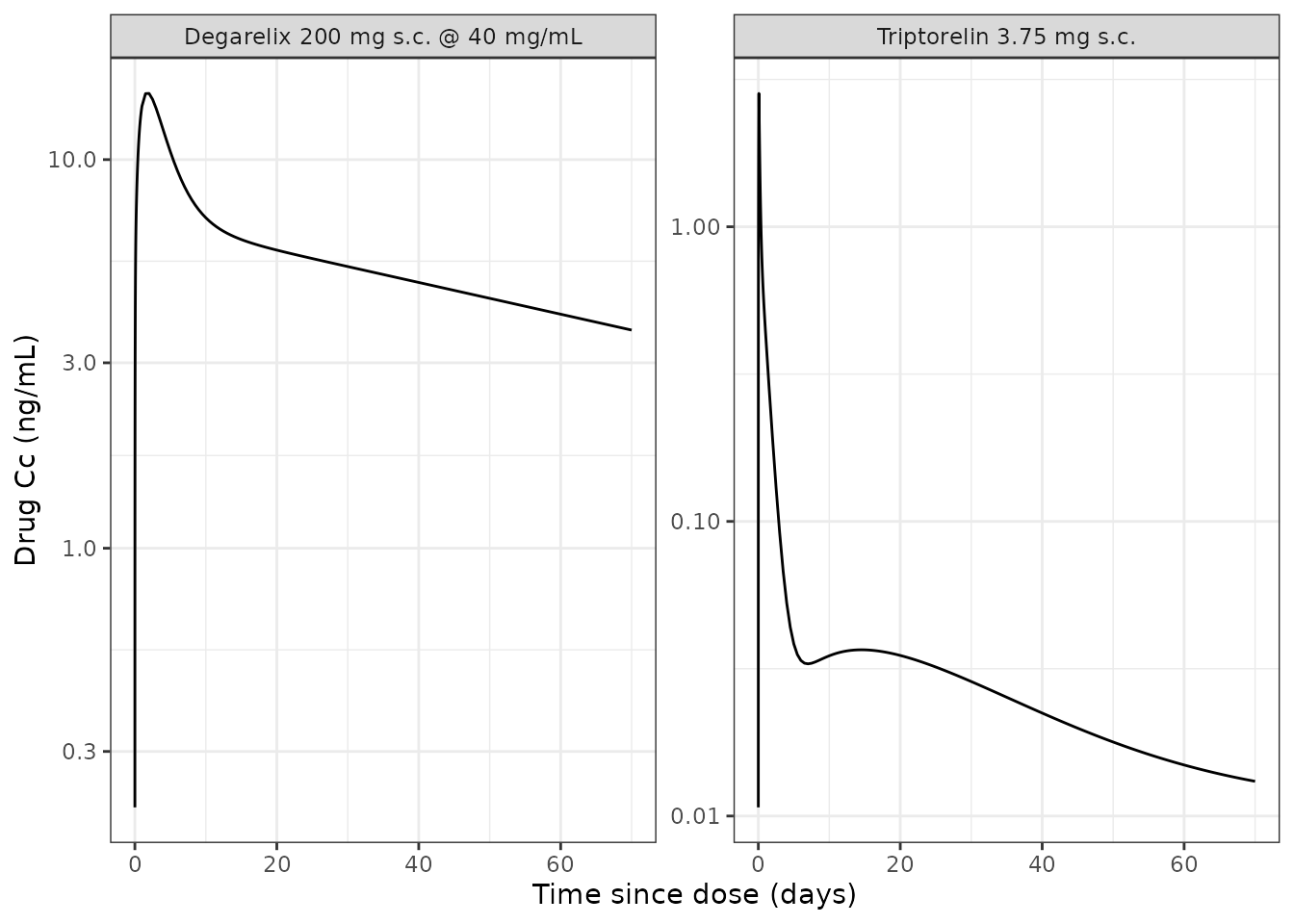
Replicates Figure 4 of Tornoe 2007 (top row): single-dose plasma drug Cc on a semilogarithmic scale.
Figure 4 (middle and bottom rows): LH and testosterone
pd_df <- bind_rows(
  tibble::tibble(time_d = sim_trip$time / 24,
                 LH = sim_trip$LH, Te = sim_trip$Te,
                 drug = "Triptorelin 3.75 mg s.c."),
  tibble::tibble(time_d = sim_deg$time / 24,
                 LH = sim_deg$LH, Te = sim_deg$Te,
                 drug = "Degarelix 200 mg s.c. @ 40 mg/mL")
) |>
  pivot_longer(c(LH, Te), names_to = "hormone", values_to = "value") |>
  filter(value > 0)

pd_df |>
  ggplot(aes(time_d, value, colour = drug)) +
  geom_line() +
  geom_hline(data = tibble::tibble(hormone = "Te", castration = 0.5),
             aes(yintercept = castration), linetype = "dotted") +
  facet_wrap(~hormone, scales = "free_y", ncol = 1,
             labeller = as_labeller(c(LH = "LH (IU/L)",
                                      Te = "Testosterone (ng/mL)"))) +
  scale_y_log10() +
  labs(x = "Time since dose (days)", y = NULL, colour = "Treatment") +
  theme_bw() +
  theme(legend.position = "bottom")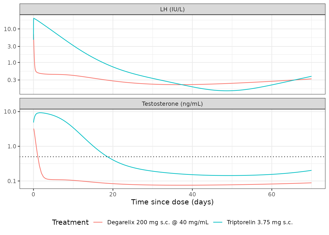
Replicates Figure 4 of Tornoe 2007 (middle = LH, bottom = testosterone). The dotted horizontal line is the 0.5 ng/mL castration threshold drawn in the published figure.
Population variability VPC (triptorelin)
A small virtual cohort illustrates between-subject variability of the triptorelin PK and HPG-axis PD response. We use 20 subjects to keep the vignette under the 5-minute render budget.
set.seed(2026)
mod_trip <- readModelDb("Tornoe_2006_triptorelin")
n_sub_vpc <- 20L

obs_grid_vpc <- c(seq(0, 1, by = 0.1),
                  seq(2, 24, by = 1),
                  seq(48, 24 * 70, by = 24))

ev_trip_vpc <- do.call(rbind, lapply(seq_len(n_sub_vpc), function(i)
  make_trip_events(dose_mg = 3.75, times = obs_grid_vpc, id = i)))

sim_trip_vpc <- as.data.frame(
  rxode2::rxSolve(mod_trip, ev_trip_vpc)
)
#> ℹ parameter labels from comments will be replaced by 'label()'

vpc_summary <- sim_trip_vpc |>
  group_by(time) |>
  summarise(across(c(Cc, LH, Te),
                   list(q05 = ~quantile(.x, 0.05, na.rm = TRUE),
                        q50 = ~quantile(.x, 0.50, na.rm = TRUE),
                        q95 = ~quantile(.x, 0.95, na.rm = TRUE)),
                   .names = "{.col}_{.fn}"),
            .groups = "drop") |>
  mutate(time_d = time / 24)

vpc_long <- vpc_summary |>
  pivot_longer(-c(time, time_d),
               names_to = c("output", "stat"),
               names_sep = "_") |>
  pivot_wider(names_from = stat, values_from = value)

ggplot(vpc_long, aes(time_d)) +
  geom_ribbon(aes(ymin = q05, ymax = q95), alpha = 0.25) +
  geom_line(aes(y = q50)) +
  facet_wrap(~output, scales = "free_y", ncol = 1,
             labeller = as_labeller(c(Cc = "Triptorelin Cc (ng/mL)",
                                      LH = "LH (IU/L)",
                                      Te = "Testosterone (ng/mL)"))) +
  scale_y_log10() +
  labs(x = "Time since dose (days)", y = NULL,
       title = "Triptorelin 3.75 mg s.c.: 5-50-95 percentiles") +
  theme_bw()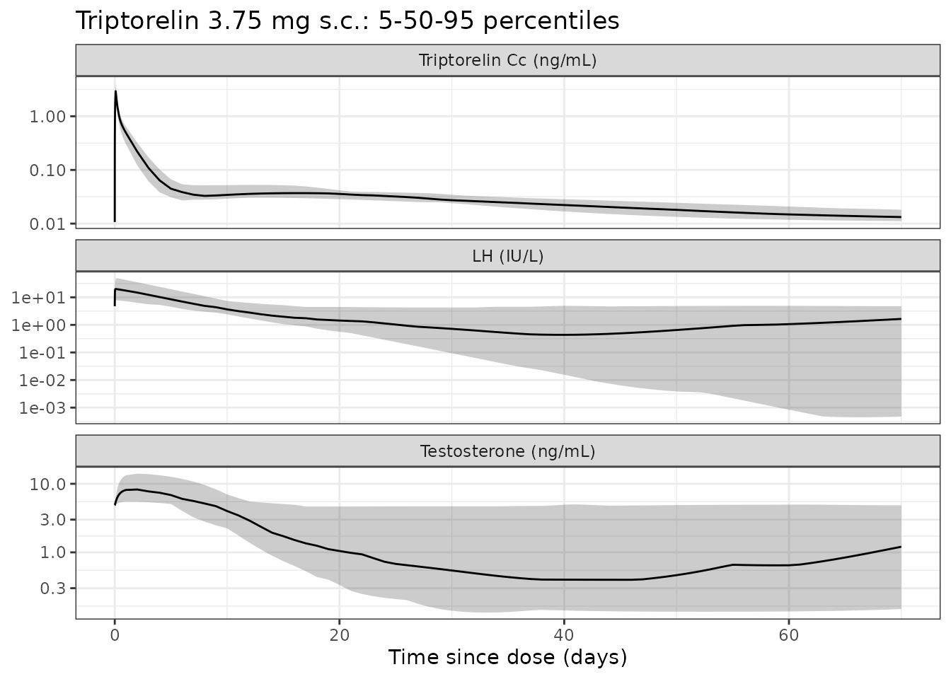
Triptorelin 3.75 mg s.c.: 5-50-95 percentiles across 20 simulated subjects.
PKNCA validation (triptorelin Cc)
Apply standard non-compartmental analysis to the typical-value triptorelin Cc profile. Tornoe 2007 does not tabulate per-arm NCA parameters, so this section confirms internal consistency rather than comparing to a published table.
sim_nca_trip <- sim_trip |>
  dplyr::filter(!is.na(Cc)) |>
  dplyr::transmute(id = 1L, time = time, Cc = Cc, treatment = "trip_3.75mg_sc")

# Guarantee a time = 0 row (pre-dose Cc = base_trip = 0.0107 ng/mL).
sim_nca_trip <- dplyr::bind_rows(
  sim_nca_trip,
  sim_nca_trip |> dplyr::distinct(id, treatment) |>
    dplyr::mutate(time = 0, Cc = 0.0107)
) |>
  dplyr::distinct(id, treatment, time, .keep_all = TRUE) |>
  dplyr::arrange(id, treatment, time)

conc_obj <- PKNCA::PKNCAconc(sim_nca_trip,
                             Cc ~ time | treatment + id)
dose_obj <- PKNCA::PKNCAdose(
  tibble::tibble(id = 1L, time = 0,
                 amt = 3.75,
                 treatment = "trip_3.75mg_sc"),
  amt ~ time | treatment + id
)
intervals <- data.frame(start = 0, end = Inf,
                        cmax = TRUE, tmax = TRUE,
                        auclast = TRUE, half.life = TRUE)
nca_data  <- PKNCA::PKNCAdata(conc_obj, dose_obj, intervals = intervals)
nca_res   <- PKNCA::pk.nca(nca_data)
nca_tbl   <- as.data.frame(nca_res$result)

knitr::kable(nca_tbl[, c("PPTESTCD", "PPORRES")],
             digits = 4,
caption = "PKNCA summary for the typical-value triptorelin profile.")| PPTESTCD | PPORRES |
|---|---|
| auclast | 76.2890 |
| cmax | 2.8346 |
| tmax | 2.0000 |
| tlast | 1680.0000 |
| lambda.z | 0.0004 |
| r.squared | 0.9999 |
| adj.r.squared | 0.9999 |
| lambda.z.time.first | 1644.0000 |
| lambda.z.time.last | 1680.0000 |
| lambda.z.n.points | 4.0000 |
| clast.pred | 0.0131 |
| half.life | 1555.3551 |
| span.ratio | 0.0231 |
Alternative degarelix dose-concentration sets
The packaged degarelix model file uses the 40 mg/mL parameter set.
The 20 and 60 mg/mL alternatives from Tornoe 2007 Table 3 are tabulated
below; users may override the corresponding ini() entries
before simulating.
| Parameter | 20 mg/mL | 40 mg/mL (packaged) | 60 mg/mL |
|---|---|---|---|
| Fr | 0.129 | 0.0573 | 0.0417 |
| F | 0.397 | 0.240 | 0.198 |
| t_1/2,slow | 53.3 d | 73.7 d | 95.4 d |
| ka,slow | 5.420e-4 /h | 3.919e-4 /h | 3.025e-4 /h |
Assumptions and deviations
- The triptorelin model file covers the s.c. arm only of the Tornoe 2007 triptorelin study. The i.m. arm (28 subjects, t_1/2,im = 17.0 days, first-order absorption, no lymphatic delay) is documented in Table 3 but not implemented; a user wishing to reproduce the i.m. data would replace the depot -> transit1 -> central pathway with a single first-order depot -> central path with ka,im = ln(2) / (17.0 * 24) = 0.001699 /h.
- The degarelix model file uses the 40 mg/mL
dose-concentration parameters as the typical value because the 200 mg @
40 mg/mL arm is the headline dose group in Figures 4-6. The 20 and 60
mg/mL alternatives are tabulated above and can be substituted by
overriding the corresponding
ini()entries before simulating. - The triptorelin baseline plasma concentration “Base” (0.0107 ng/mL, Table 3) is interpreted as an additive offset on the predicted triptorelin Cc rather than as a residual-error-model parameter. This matches the symbol’s definition in the paper’s “Definition of terms” section (“base, triptorelin baseline”) and the proximity to the triptorelin assay LLOQ of 0.01 ng/mL.
- The published logit-scale IIVs for Fr and F follow
the paper’s approximation
CV(q) = (1 - q) * w_q, wherew_qis the underlying SD on the logit scale. The packaged values are(CV(q) / (1 - q))^2, matching the paper’s Table 3 IIV CV(%) for each parameter at the reported typical-value q. - The paper used sequential PK then PD fitting, with individual predicted plasma concentrations from the PK model fed as a time-varying driver into the PD model via linear interpolation. The packaged models simulate the joint PK + PD system in a single rxode2 solve. For typical-value simulation the two approaches are equivalent; for refitting, joint estimation is now standard.
- The IIV correlations reported in the paper’s CV(%) columns are encoded as diagonal log-normal IIV variances. The paper does not report a full OMEGA correlation matrix, so off-diagonal correlations are assumed zero.
- Event tables must include explicit observation rows with
cmtmatching each output (Cc,LH,Te), as shown in themake_obs_rows()/make_trip_events()/make_deg_events()helpers. Therxode2::et()shortcut does not auto-generate observation rows for multi-output models.