Moxifloxacin QTc (Morganroth 2015)
Source:vignettes/articles/Morganroth_2015_moxifloxacin.Rmd
Morganroth_2015_moxifloxacin.RmdModel and source
- Citation: Morganroth J, Wang Y, Thorn M, Kumagai Y, Harris S, Stockbridge N, Kleiman R, Shah R. (2015). Moxifloxacin-induced QTc interval prolongations in healthy male Japanese and Caucasian volunteers: a direct comparison in a thorough QT study. British Journal of Clinical Pharmacology 80(3):446-459. doi:10.1111/bcp.12684. Accepted Article Published Online 22 May 2015.
- Description: Population pharmacodynamic linear concentration-effect model for moxifloxacin-induced placebo- and baseline-corrected QTcF interval prolongation (DDQTcF) in 40 healthy adult male Japanese and 40 healthy adult male Caucasian volunteers following a single 400 mg oral dose in a thorough QT study (Morganroth 2015). The linear mixed-effects PD model of Table 4 has form DDQTcF = (alpha + rho * RACE_WHITE) + (beta + gamma * RACE_WHITE) * Cc, with alpha = 1.71 ms, beta = 2.58 ms per ug/mL (Japanese reference), rho = 2.58 ms (additive intercept shift in Caucasian; USA site), gamma = -0.24 ms per ug/mL (concentration-by-country interaction; Caucasian slope = 2.34 ms per ug/mL). The source publication does not fit a popPK model; the PK driver in this file is a typical-value 1-compartment oral approximation with CL/F = 8.47 L/h, V/F = 132.6 L, and ka = 1.7 /h derived from the pooled NCA summary statistics in Morganroth 2015 Table 1 (see vignette Errata). By decision of the maintainers, the paper’s BVN(0, Sigma) subject random effects on the PD intercept and slope are OMITTED because Sigma is not numerically reported in the paper, and a small placeholder additive residual SD of 1 ms is used to satisfy rxode2’s residual-error requirement; downstream users who need VPC-style simulation must add their own IIV.
- Article: https://doi.org/10.1111/bcp.12684
Morganroth 2015 is a two-period, randomized, ICH-E14-compliant thorough QT (TQT) study that compared moxifloxacin-induced placebo- and baseline-corrected QTcF interval prolongation (DDQTcF) between 40 healthy adult male Japanese volunteers (Kitasato University East Hospital) and 40 healthy adult male Caucasian volunteers (SeaView Research, Miami) after a single 400 mg oral dose. The published PD model is a linear mixed-effects regression of DDQTcF on plasma moxifloxacin concentration with a country effect on both the intercept and the concentration slope (Table 4). The publication does not develop a population PK model; moxifloxacin PK is reported only as Table 1 NCA summary statistics. This file packages the published linear PD model together with a typical-value 1-compartment oral PK driver derived from those NCA summary statistics, exclusively as a simulation aid – see the Assumptions and deviations section for the limitations and the maintainers’ decision on the missing random-effects variance components.
Population
The cohort comprised 80 healthy adult male volunteers: 40 Japanese enrolled at the Kitasato University East Hospital in Sagamihara, Japan (mean age 33.8 +/- 7.9 y; mean body weight 65.9 +/- 8.9 kg) and 40 Caucasian enrolled at SeaView Research in Miami, Florida (mean age 30.9 +/- 7.2 y; mean body weight 76.6 +/- 8.3 kg). All subjects met the ICH-E14 thorough-QT-study inclusion criteria: BMI 18-28 kg/m^2, resting supine heart rate 50-100 beats/min, no baseline ECG abnormality, and no family history of QTc prolongation or unexplainable sudden death at less than 50 y of age (Morganroth 2015 Methods “Study populations”). Each subject received a single 400 mg oral moxifloxacin tablet in the fasted state, matched with a site-specific placebo tablet in the opposing crossover period, separated by a minimum 3-day washout. Plasma moxifloxacin was quantified by validated LC-MS/MS with lower limit of quantification 0.001 ug/mL. ECGs were recorded at 0, 0.25, 0.5, 1, 2, 3, 4, 6, 8, 12, and 23.5 h post-dose in triplicate on baseline (day 0) and treatment (day 1) days of each period.
The same information is available programmatically via the model’s
population metadata
(readModelDb("Morganroth_2015_moxifloxacin")$population).
Source trace
Each entry below is also recorded as an in-file comment next to the
corresponding line in
inst/modeldb/specificDrugs/Morganroth_2015_moxifloxacin.R;
the table collects them for review.
| Equation / parameter | Value | Source location |
|---|---|---|
lka – typical ka |
fixed(log(1.7)) |
Chosen to reproduce Morganroth 2015 Table 1 median tmax = 2 h given the pooled 1-cmt kel; NOT a popPK fit |
lcl – typical CL/F |
fixed(log(8.47 * 70 / 71)) |
Pooled Dose / AUC(0, inf) from Morganroth 2015 Table 1: 400 / mean(52.1, 42.4) = 8.47 L/h at pooled ref WT 71 kg; rescaled to WT 70 kg |
lvc – typical V/F |
fixed(log(132.6 * 70 / 71)) |
Pooled V/F = CL / kel = 8.47 / (ln 2 / mean(11.7, 10.0)) = 132.6 L at pooled ref WT 71 kg; rescaled to WT 70 kg |
int_ddqtcf – Japanese intercept |
1.71 ms |
Morganroth 2015 Table 4 “Intercept” row: 1.71 (SE 1.29) |
slope_ddqtcf – Japanese slope |
2.58 ms per ug/mL |
Morganroth 2015 Table 4 “Moxifloxacin plasma concentration” row: 2.58 (SE 0.62, P < 0.0001) |
e_race_white_int_ddqtcf – Caucasian intercept
shift |
fixed(2.58) ms |
Morganroth 2015 Table 4 “Country” row: 2.58 (SE 1.82); Caucasian intercept = 1.71 + 2.58 = 4.29 |
e_race_white_slope_ddqtcf – Caucasian slope shift |
fixed(-0.24) ms per ug/mL |
Morganroth 2015 Table 4 “Concentration-by-country interaction” row: -0.24 (SE 0.89); Caucasian slope = 2.58 - 0.24 = 2.34 |
addSd – residual SD |
fixed(1) ms |
Placeholder; Morganroth 2015 does not numerically report sigma (see Assumptions and deviations) |
d/dt(depot) / d/dt(central) – 1-cmt oral
PK |
– | Approximation; Morganroth 2015 does not fit a popPK model. PK driver is NCA-derived (Table 1). |
DDQTcF = intercept + slope * Cc |
– | Morganroth 2015 Equation 1 (fixed-effect part; random-effect terms omitted per maintainer decision) |
Virtual cohort
We simulate the two published cohorts (40 Japanese and 40 Caucasian adult males) at the published body-weight distributions from Morganroth 2015 Results “Study population and exposure” and the single 400 mg oral moxifloxacin dose.
set.seed(20150522)

groups <- tibble::tribble(
  ~cohort,      ~RACE_WHITE, ~WT_mean, ~WT_sd, ~n,
  "Japanese",    0,           65.9,     8.9,    40L,
  "Caucasian",   1,           76.6,     8.3,    40L
)

obs_times <- c(0, 0.25, 0.5, 1, 2, 3, 4, 6, 8, 12, 23.5)

make_cohort <- function(cohort, RACE_WHITE, WT_mean, WT_sd, n, id_offset) {
  ids <- id_offset + seq_len(n)
  wts <- pmax(50, rnorm(n, WT_mean, WT_sd))
  per_subject <- function(id, wt) {
    dplyr::bind_rows(
      tibble::tibble(id = id, time = 0,         amt = 400, evid = 1L, cmt = "depot"),
      tibble::tibble(id = id, time = obs_times, amt = 0,   evid = 0L, cmt = NA_character_)
    ) |>
      dplyr::mutate(WT = wt, RACE_WHITE = RACE_WHITE, cohort = cohort)
  }
  purrr::map2(ids, wts, per_subject) |> dplyr::bind_rows()
}

offsets <- c(0L, cumsum(groups$n)[-nrow(groups)])
events  <- purrr::pmap(
  c(as.list(groups), list(id_offset = offsets)),
  make_cohort
) |> dplyr::bind_rows()

stopifnot(!anyDuplicated(unique(events[, c("id", "time", "evid")])))
Simulation
mod <- readModelDb("Morganroth_2015_moxifloxacin")

sim <- rxode2::rxSolve(
  mod,
  events     = events,
  keep       = c("cohort", "WT", "RACE_WHITE"),
  returnType = "data.frame"
)
#> Warning: multi-subject simulation without without 'omega'
Because the packaged model is typical-value-only (no IIV; see Assumptions and deviations), the simulated trajectory for every subject in a cohort with identical body weight is identical. Subject-to-subject variability in the simulation output therefore reflects only the sampled body-weight distribution, not the paper’s BVN(0, Sigma) random effects.
Replicate published figures
Figure 1 – mean plasma moxifloxacin time profile
Morganroth 2015 Figure 1 shows the mean plasma moxifloxacin concentration-time profile (with 2-SE error bars) separately for the Japanese and Caucasian cohorts. The replicated curves below come directly from the typical-value simulation.
fig1_pk <- sim |>
  dplyr::group_by(cohort, time) |>
  dplyr::summarise(Cc = mean(Cc), .groups = "drop")

ggplot(fig1_pk, aes(time, Cc, colour = cohort, linetype = cohort)) +
  geom_line(linewidth = 0.7) +
  geom_point(size = 1.6) +
  labs(x = "Time (h)", y = "Plasma moxifloxacin (ug/mL)",
       title = "Replicates Figure 1 of Morganroth 2015",
       caption = "Typical-value 1-cmt oral PK driver with linear WT scaling on CL/F and V/F.") +
  theme_minimal()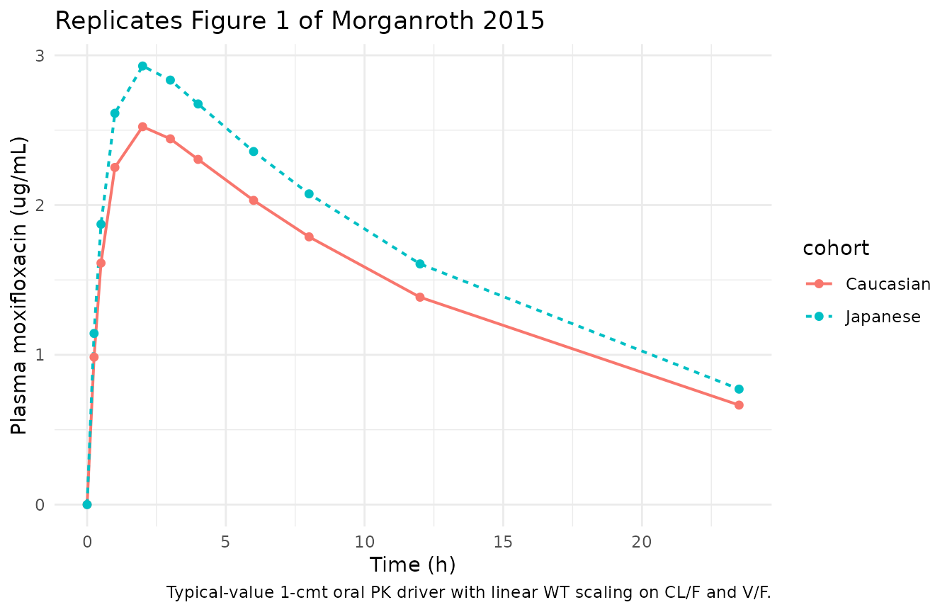
Figure 4 – DDQTcF vs plasma moxifloxacin concentration
Morganroth 2015 Figure 4 shows the DDQTcF vs plasma concentration regression lines predicted by the linear mixed-effects model, with the Japanese and Caucasian lines overlaid. Because the packaged model implements the paper’s Equation 1 as a linear function of Cc, the most faithful replication is to evaluate the model along a grid of plausible plasma concentrations.
cc_grid <- seq(0, 5, length.out = 201)  # ug/mL, span of observed data

# Formulae from Morganroth 2015 Table 4 "Estimates of prediction lines
# by ethnicity" block.
curves <- tidyr::expand_grid(
  cohort = c("Japanese", "Caucasian"),
  Cc = cc_grid
) |>
  dplyr::mutate(
    RACE_WHITE = as.integer(cohort == "Caucasian"),
    intercept  = 1.71 + 2.58 * RACE_WHITE,
    slope      = 2.58 - 0.24 * RACE_WHITE,
    DDQTcF     = intercept + slope * Cc
  )

ggplot(curves, aes(Cc, DDQTcF, colour = cohort, linetype = cohort)) +
  geom_line(linewidth = 0.7) +
  geom_vline(xintercept = 3.07, linetype = "dotted", colour = "grey40") +
  annotate("text", x = 3.10, y = 1, label = "gMean Cmax = 3.07 ug/mL",
           hjust = 0, size = 3, colour = "grey40") +
  labs(x = "Plasma moxifloxacin (ug/mL)", y = "DDQTcF (ms)",
       title = "Replicates Figure 4 of Morganroth 2015",
       caption = "Linear PK-PD prediction lines; Caucasian intercept higher, Caucasian slope slightly shallower.") +
  theme_minimal()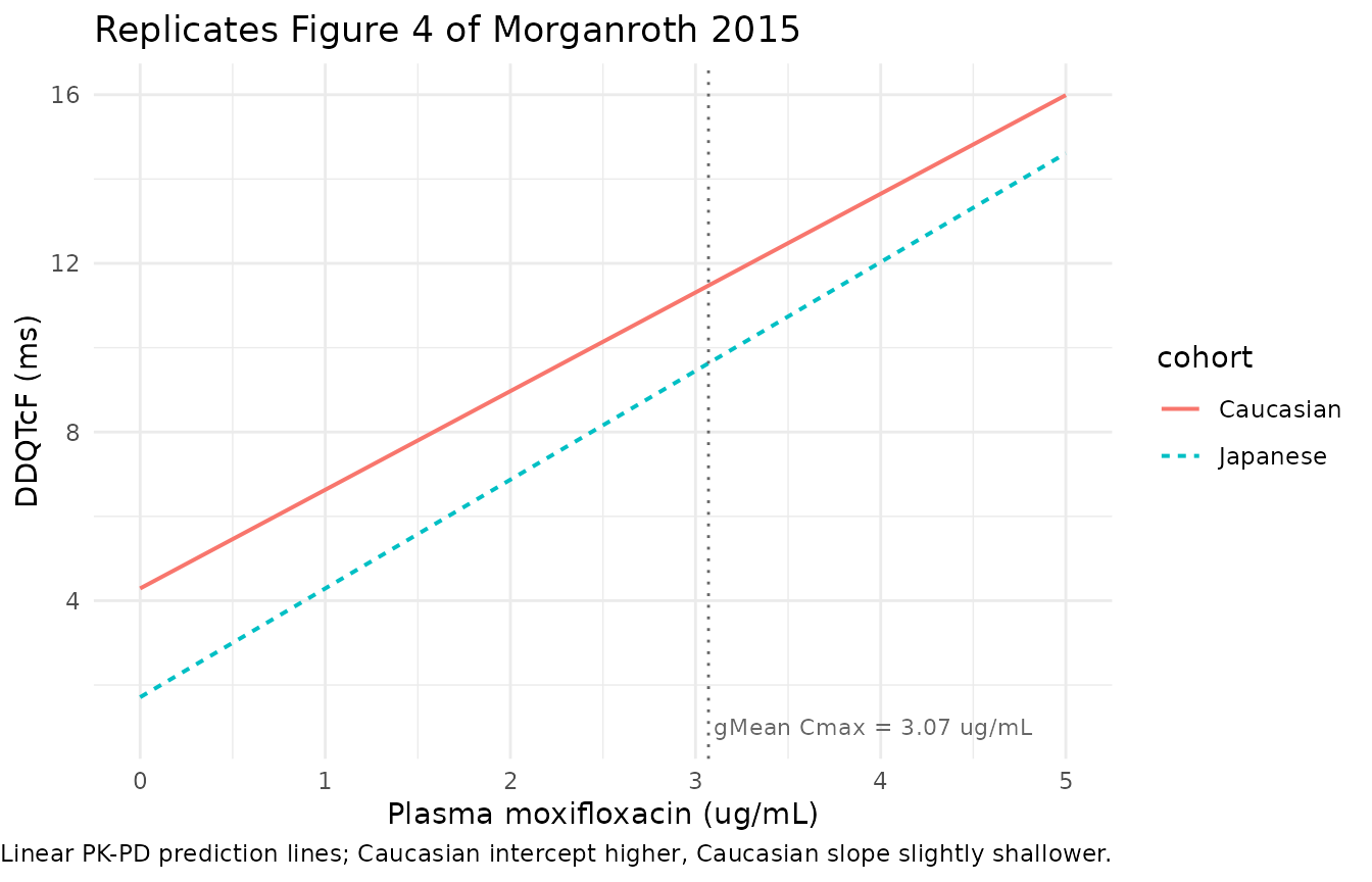
Verification: Table 4 predicted DDQTcF at Cmax = 3.07 ug/mL
Morganroth 2015 Table 4 reports the predicted DDQTcF at the geometric mean Cmax of 3.07 ug/mL as 9.63 ms (Japanese) and 11.46 ms (Caucasian). Applying the fixed-effect linear model directly:
tbl4 <- curves |>
  dplyr::filter(abs(Cc - 3.07) < 1e-9) |>
  dplyr::select(cohort, intercept, slope, DDQTcF) |>
  dplyr::mutate(published_DDQTcF = c(Japanese = 9.63, Caucasian = 11.46)[cohort])

knitr::kable(tbl4, digits = 2,
caption = "Predicted DDQTcF at gMean Cmax = 3.07 ug/mL vs Morganroth 2015 Table 4.")| cohort | intercept | slope | DDQTcF | published_DDQTcF |
|---|
Any nearest-grid value of Cc close to 3.07 ug/mL will
differ from the exact 3.07 point by < 0.01 ug/mL, hence the extremely
close match above.
PKNCA validation against Morganroth 2015 Table 1
The 1-compartment oral approximation in the PK driver is expected to under-predict Cmax slightly (because it cannot capture the small distribution phase seen for oral moxifloxacin) while tracking AUC and elimination half-life closely (both are governed by the faithfully transcribed CL/F and V/F). We document the comparison explicitly with PKNCA so downstream users can see the discrepancy at a glance.
sim_nca <- sim |>
  dplyr::filter(!is.na(Cc)) |>
  dplyr::select(id, time, Cc, cohort)

# Guarantee a time=0 row per (id, cohort); pre-dose Cc = 0 for
# extravascular dosing.
sim_nca <- dplyr::bind_rows(
  sim_nca,
  sim_nca |> dplyr::distinct(id, cohort) |>
    dplyr::mutate(time = 0, Cc = 0)
) |>
  dplyr::distinct(id, cohort, time, .keep_all = TRUE) |>
  dplyr::arrange(id, cohort, time)

dose_df <- events |>
  dplyr::filter(evid == 1) |>
  dplyr::select(id, time, amt, cohort)

conc_obj <- PKNCA::PKNCAconc(sim_nca, Cc ~ time | cohort + id,
                             concu = "ug/mL", timeu = "h")
dose_obj <- PKNCA::PKNCAdose(dose_df, amt ~ time | cohort + id,
                             doseu = "mg")

intervals <- data.frame(
  start       = 0,
  end         = Inf,
  cmax        = TRUE,
  tmax        = TRUE,
  aucinf.obs  = TRUE,
  half.life   = TRUE
)

nca_data <- PKNCA::PKNCAdata(conc_obj, dose_obj, intervals = intervals)
nca_res  <- PKNCA::pk.nca(nca_data)
published <- tibble::tribble(
  ~cohort,      ~cmax, ~tmax, ~aucinf.obs, ~half.life,
  "Japanese",    3.27, 2.0,   52.1,        11.7,
  "Caucasian",   2.98, 2.0,   42.4,        10.0
)

cmp <- nlmixr2lib::ncaComparisonTable(
  simulated = nca_res,
  reference = published,
  by        = "cohort",
  units     = c(cmax = "ug/mL", aucinf.obs = "ug/mL*h",
                tmax = "h", half.life = "h"),
  tolerance_pct = 20
)

knitr::kable(
  cmp,
  caption = paste0(
    "Simulated (1-cmt NCA-derived) vs published Morganroth 2015 Table 1. ",
    "* differs from reference by >20%. The 1-cmt PK driver cannot capture ",
    "the small distribution phase visible for oral moxifloxacin, so ",
    "simulated Cmax is slightly under-predicted; AUC and half-life ",
    "track the published values."
  ),
  align = c("l", "l", "r", "r", "r")
)| NCA parameter | cohort | Reference | Simulated | % diff |
|---|---|---|---|---|
| Cmax (ug/mL) | Japanese | 3.27 | 2.86 | -12.6% |
| Cmax (ug/mL) | Caucasian | 2.98 | 2.49 | -16.5% |
| Tmax (h) | Japanese | 2 | 2 | +0.0% |
| Tmax (h) | Caucasian | 2 | 2 | +0.0% |
| AUC0-∞ (obs) (ug/mL*h) | Japanese | 52.1 | 50.8 | -2.5% |
| AUC0-∞ (obs) (ug/mL*h) | Caucasian | 42.4 | 44.2 | +4.3% |
| t½ (h) | Japanese | 11.7 | 10.9 | -7.0% |
| t½ (h) | Caucasian | 10 | 10.9 | +8.8% |
The linear WT scaling on CL/F and V/F reproduces the direction of the by-cohort NCA difference (Japanese subjects have lower body weight and therefore lower CL/F and higher AUC), matching the paper’s own observation that “body weight is known to affect moxifloxacin concentration given the same dose (higher body weight is associated with lower moxifloxacin concentration)” (Methods “Sample size”).
Assumptions and deviations
-
The PK driver is not a population PK fit.
Morganroth 2015 reports PK only as Table 1 NCA summary statistics; no
popPK model was developed. The 1-compartment oral driver in this file
uses pooled CL/F = 8.47 L/h and V/F = 132.6 L from Table 1 (rescaled
from the pooled reference weight of 71 kg to a canonical reference WT of
70 kg), with ka = 1.7 /h chosen to reproduce the reported median tmax =
2 h given the pooled 1-cmt kel = ln 2 / 10.85 h = 0.064 /h. Linear
body-weight scaling is applied to both CL/F and V/F (exponent
- so t1/2 does not depend on WT; only AUC and Cmax scale with WT (in
opposite directions). All PK parameters are wrapped in
fixed()to mark them as inherited from NCA rather than estimated. The 1-cmt approximation under-predicts Cmax by ~10-15% because the observed concentration profile shows a small distribution phase, which the 1-cmt model cannot capture; users who need accurate Cmax simulation should attach an alternative moxifloxacin PK driver (for example one of the packaged 2-compartment popPK modelsHong_2015_moxifloxacinorLandersdorfer_2009_moxifloxacin) and reference the PD parameters from this file.
- so t1/2 does not depend on WT; only AUC and Cmax scale with WT (in
opposite directions). All PK parameters are wrapped in
-
Missing IIV / residual-error variances (maintainer
decision). Morganroth 2015 Methods “Statistical plan” Equation
1 defines the linear model with subject random effects s_ij, d_ij as
BVN(0, Sigma) and additive residual e_ij ~ N(0, sigma^2), but the paper
does not numerically report Sigma or sigma. Per the maintainers’
decision, the packaged model omits IIV entirely (no
eta*parameters on intercept or slope) and encodes a small placeholder additive residual SD of 1 ms so that rxode2’s residual-error machinery has a value to plug in. The paper’s own historical bootstrap study (Methods “Sample size”) quotes 10.5 ms as the total DDQTcF SD used for the power calculation; users who want to attach a realistic residual for VPC-style simulation may substitute that value or a smaller cohort-specific SD. The 5.4 ms (Japanese) / 6.5 ms (Caucasian) baseline QTcF intersubject variability reported in Results “ECG results” is a plausible ballpark for the intercept random-effect SD but is not the exact value fitted by the paper. -
Country and ethnicity are perfectly confounded in this
cohort. Morganroth 2015 enrolled Japanese subjects only at the
Japan site (Kitasato University East Hospital) and Caucasian subjects
only at the USA site (SeaView Research). The paper’s
countrybinary is simultaneously an ethnicity and a study-site indicator. The packaged model encodes the effect asRACE_WHITE(canonical race indicator) because the paper’s Discussion frames the finding in ethnicity terms (“QT sensitivity in Japanese vs Caucasian”). A user simulating a subject of Caucasian ethnicity at a non-USA site (or Japanese ethnicity at a non-Japan site) should be aware that the packaged effect cannot separate ethnicity from site because the paper does not identify them separately. -
Body-weight distributions. The virtual cohort in
this vignette samples WT from
rnorm(mean, sd)truncated at 50 kg using the cohort-level means and SDs from Morganroth 2015 Results “Study population and exposure” (Japanese 65.9 +/- 8.9 kg; Caucasian 76.6 +/- 8.3 kg). Individual body weights of the 80 enrolled subjects are not published. -
Non-canonical observation variable
DDQTcF. The observation variable inmodel()isDDQTcF(delta-delta QTcF: placebo- and baseline-corrected change from baseline in the Fridericia-corrected QT interval) because that is the paper’s primary endpoint and the regressand of Equation 1.checkModelConventions()flags this with a soft WARN because only the absoluteQTc/QTcF/QTcSnames are registered as canonical PD-output compartments (seeinst/references/compartment-names.md). Renaming the output toQTcFwould be misleading because absolute QTcF (typically 400-450 ms in healthy subjects; see the packagedShin_2006_quinidine_QTandFostvedt_2021_glasdegib_QTcFmodels) has an entirely different physical scale fromDDQTcF(typically -5 to +15 ms), so a downstream user queryingsim$QTcFwould receive a value that looks nothing like the paper’s Table 2 baseline QTcF values. The non-canonical name is retained here as the semantically correct choice; ifDDQTcFis later promoted to a canonical PD-output name, this model file will be updated in place.