Model and source
- Citation: Zhang S, Amrite A, Tan B, Jamsen K, Pradhan S, Choy S, Plotkin H. Nedosiran population pharmacokinetic and pharmacodynamic modelling and simulation to guide clinical development and dose selection in patients with primary hyperoxaluria type 1. Br J Clin Pharmacol. 2024;90(12):3176-3189. doi:10.1111/bcp.16194
- Description: Two-compartment population PK/PD model for nedosiran (GalNAc-conjugated siRNA targeting hepatic LDHA) in healthy volunteers and patients with primary hyperoxaluria, with dual parallel n-transit subcutaneous absorption (a 2-compartment slow chain and a 4-compartment fast chain), parallel linear and Michaelis-Menten elimination, and an effect-compartment-driven sigmoid-Imax indirect-response model inhibiting production of 24-h urinary oxalate; developed from 1978 plasma concentrations in 143 participants and 588 24-h urinary oxalate observations in 46 PH1 patients across five clinical studies (Zhang 2024).
- Article: https://doi.org/10.1111/bcp.16194
Nedosiran (RIVFLOZA) is a GalNAc-conjugated small interfering RNA that silences hepatic LDHA, the gene encoding the lactate dehydrogenase isoform responsible for the terminal glyoxylate-to-oxalate step in the liver. Zhang 2024 pooled five clinical studies (PHYOX1, PHYOX2, PHYOX3, PHYOX5, PHYOX6) into a single population PK/PD analysis and used it to confirm the approved weight-banded dosing regimen.
The model is one jointly developed PK/PD analysis and is therefore packaged as a single model file.
Structure
The structure below is taken from Zhang 2024 Figure 3 (page 3183). The number of transit compartments in each absorption chain appears nowhere in the text or in either parameter table – it is only readable from the Figure 3 schematic:
-
Slow pathway (fraction
FR1of the dose): input compartmentdepot1– ka1 –>transit1– ka1 –>central(two states in series). -
Fast pathway (fraction
1 - FR1): input compartmentdepot2– ka2 –>transit2– ka2 –>transit3– ka2 –>transit4– ka2 –>central(four states in series).
So the paper’s “dual n-transit absorption” is n = 2
for the slow pathway and n = 4 for the fast pathway.
Disposition is two-compartment with parallel linear
(CL/F) and Michaelis-Menten
(Vmax * C / (KM + C)) elimination from
central; the paper attributes the linear arm to renal
elimination and the saturable arm to ASGPR-mediated hepatic uptake. A
Sheiner effect compartment with ke0 = ln(2) / lambda drives
a sigmoid-Imax indirect-response model that inhibits production of 24-h
urinary oxalate.
Population
The PK dataset comprised 1978 plasma nedosiran concentrations from 143 participants: 85 healthy adult volunteers without a primary hyperoxaluria (PH) diagnosis, 46 patients with PH type 1 (PH1) and 12 with PH2. The PD dataset comprised 588 24-h urinary oxalate observations from the 46 PH1 patients in PHYOX1, PHYOX2 and PHYOX3, adjusted per 1.73 m^2 body surface area in participants aged under 18 years. Placebo-arm PD data (n = 11) were excluded after showing no apparent change over 28 weeks, and 13.1% of PK observations fell below the 1.0 ng/mL LLOQ and were excluded.
Doses spanned 1.5, 3.0 and 6.0 mg/kg single subcutaneous doses
(PHYOX1, PHYOX6), a 170 mg single dose (PHYOX5), and repeat once-monthly
flat doses of 170 mg (nedosiran sodium salt; 160 mg free-acid
equivalent) or 136 mg for body weight below 50 kg (PHYOX2, PHYOX3). All
participants with eGFR below 30 mL/min/1.73 m^2 were non-PH volunteers
from PHYOX5. Baseline demographics are tabulated in Supporting
Information Table S1, which is not available to this extraction; the
population metadata records that gap explicitly rather than
substituting values.
str(rxode2::rxode(readModelDb("Zhang_2024_nedosiran"))$population)
#> ℹ parameter labels from comments will be replaced by 'label()'
#> List of 11
#>  $ species       : chr "human"
#>  $ n_subjects    : int 143
#>  $ n_studies     : int 5
#>  $ age_range     : chr "adults and children aged >= 6 years (14 participants aged 9 to <18 years contributed PK, 10 contributed PD); ex"| __truncated__
#>  $ weight_range  : chr "not reported in the main text (Supporting Information Table S1); the simulation reference subject is 70 kg and "| __truncated__
#>  $ sex_female_pct: num NA
#>  $ disease_state : chr "85 healthy adult volunteers without a primary hyperoxaluria diagnosis, 46 patients with primary hyperoxaluria t"| __truncated__
#>  $ dose_range    : chr "1.5, 3.0 or 6.0 mg/kg single s.c. dose (PHYOX1, PHYOX6); 170 mg s.c. single dose (PHYOX5); repeat flat s.c. dos"| __truncated__
#>  $ regions       : chr "not reported in the main text; PHYOX6 was an ethno-bridging study in Japanese and Caucasian healthy adults"
#>  $ renal_function: chr "eGFR spanned normal through end-stage renal disease; all participants with eGFR <30 mL/min/1.73 m^2 were non-PH"| __truncated__
#>  $ notes         : chr "PK: 1978 plasma nedosiran concentrations from 143 participants across PHYOX1, PHYOX2, PHYOX3, PHYOX5 and PHYOX6"| __truncated__
Source trace
Every ini() entry in
inst/modeldb/specificDrugs/Zhang_2024_nedosiran.R carries
an in-file comment naming its source. They are collected here for
review.
| Equation / parameter | Value | Source location |
|---|---|---|
lcl (CL/F) |
5.69 L/h | Table 1 |
lvc (Vc/F) |
147 L | Table 1 |
lq (Q/F) |
2.45 L/h | Table 1 |
lvp (Vp/F) |
5300 L | Table 1 |
lvmax (Vmax) |
3.94 mg/h | Table 1 |
lkm (KM) |
293 ng/mL | Table 1 |
logitffo (FR1) |
69.80% | Table 1 |
lka1 |
0.22 1/h | Table 1 |
lka2 |
16.7 1/h | Table 1 |
e_wt_cl |
0.75 FIX | Table 1 (“Exponent for WT on CL/F and Q/F”) |
e_wt_vc |
1 FIX | Table 1 (“Exponent for WT on Vc/F and Vp/F”) |
e_crcl_cl |
0.87 | Table 1 (“Exponent for eGFR on CL/F”) |
e_crcl_vc |
0.19 | Table 1 (“Exponent for eGFR on Vc/F”) |
e_wt_ka |
0.83 | Table 1 (“Exponent for WT on ka1 and ka2”) |
e_dis_ph1_ka1 |
1.54 | Table 1 (“Covariate effect of PH1 on ka1”) |
lrbase (baseline Uox) |
1420 umol/24 h | Table 2 |
lkout (Kout) |
0.338 1/week | Table 2 (converted to 1/h by /168) |
logitimax (Imax) |
64.5% | Table 2 |
lic50 (IC50) |
1.04 ng/mL | Table 2 |
lhill (gamma) |
2.56 | Table 2 |
lke0 |
ln(2) / 21.9 weeks | Table 2 (lambda = 21.9 weeks); Figure 3
(ke0 = ln(2)/lambda) |
etalvc, etalka1, etalka2,
etalvmax
|
27.1, 42.1, 27.6, 35.3 %CV | Table 1 |
etalogitffo |
0.35 (additive) | Table 1 – see “Recovering the variability scale” |
etalrbase, etalic50,
etalogitimax
|
31.7, 86, 29.4 %CV | Table 2 |
propSd |
27.70% | Table 1; Results 3.2 (“additive on the log-scale … equates to a proportional RUV on the normal scale”) |
addSd_uox |
205 umol/24 h SD | Table 2 |
| Absorption chain lengths (2 slow, 4 fast) | n/a | Figure 3 only – absent from the text and both tables |
Eff = Imax * Ceff^gamma / (Ceff^gamma + IC50^gamma) |
n/a | Figure 3 (inset equation) |
d/dt(UO24) = kin * (1 - Eff) - kout * UO24 |
n/a | Figure 3 |
CL/F = 5.69 * (WT/70)^0.75 * (eGFR/90)^0.87 |
n/a | Results 3.2 (equation; coefficients from Table 1) |
Vc/F = 147 * (WT/70)^1 * (eGFR/90)^0.19 |
n/a | Results 3.2 |
ka1 = 0.22 * (WT/70)^0.83 * 1.54^PH1,
ka2 = 16.7 * (WT/70)^0.83
|
n/a | Results 3.2 |
Recovering the variability scale
Zhang 2024 never states the scale on which two of its variability terms were estimated, and both matter for simulation. This section documents how the ambiguity was resolved – from the paper’s own numbers, not from assumption.
The tables report standard deviations, not
variances. Table 2’s additive residual error row is labelled
explicitly (SD, umol/24 h) 205. Read as a variance it would
imply a residual SD of 14 umol/24 h against a 1420 umol/24 h baseline,
which is not credible. Every other variability entry in Tables 1 and 2
is a %CV, which the table footnote defines as the
“approximate coefficient of variation” – i.e. 100 * omega.
The one unlabelled entry,
Between-subject variability for FR1 (additive) 0.35, is
therefore also a standard deviation on FR1’s estimation scale.
That estimation scale must be bounded. FR1 = 0.698
is a dose-split fraction. An additive SD of 0.35 applied directly to it
would put about 22% of subjects outside [0, 1] and send the fast-pathway
fraction 1 - FR1 negative. The same argument applies to
Imax = 0.645 with a 29.4 %CV: log-normal on the natural scale puts
Imax > 1 for 6.8% of subjects, which drives
kin * (1 - Eff) negative and 24-h urinary oxalate below
zero. Both are carried on the logit scale in this implementation.
The Imax case is directly falsifiable against the paper’s own
simulation. Figure 5C plots the median and 95% prediction interval of
24-h urinary oxalate out to week 132; digitised from the published
figure, the plateau is approximately 245 / 485 / 990 umol/24
h. At steady state the effect-compartment concentration is far
above IC50, so Eff is within 0.2% of Imax and
the plateau reduces to rbase * (1 - Imax). That makes the
two candidate encodings separable with a few thousand draws and no ODE
solve:
set.seed(20240701)
n_draw <- 20000
rbase <- 1420 * exp(rnorm(n_draw, 0, 0.317))     # Table 2: 31.7 %CV on baseline

encodings <- list(
  "logit-normal Imax (as packaged)" = plogis(qlogis(0.645) + rnorm(n_draw, 0, 0.294)),
  "log-normal Imax (counterfactual)" = exp(log(0.645) + rnorm(n_draw, 0, 0.294))
)

scale_check <- lapply(names(encodings), function(nm) {
  uox_ss <- rbase * (1 - encodings[[nm]])
  tibble(
    encoding = nm,
    `2.5th`  = quantile(uox_ss, 0.025),
    median   = quantile(uox_ss, 0.500),
    `97.5th` = quantile(uox_ss, 0.975),
    `% below zero` = 100 * mean(uox_ss < 0)
  )
}) |>
  bind_rows() |>
  bind_rows(tibble(encoding = "Zhang 2024 Figure 5C (digitised)",
                   `2.5th` = 245, median = 485, `97.5th` = 990,
                   `% below zero` = 0))

knitr::kable(
  scale_check, digits = 1,
  caption = paste("Steady-state 24-h urinary oxalate under the two candidate",
                  "Imax variability encodings, against the plateau digitised",
                  "from Zhang 2024 Figure 5C.")
)| encoding | 2.5th | median | 97.5th | % below zero |
|---|---|---|---|---|
| logit-normal Imax (as packaged) | 239.5 | 501.6 | 1023.2 | 0.0 |
| log-normal Imax (counterfactual) | -203.2 | 486.4 | 1223.7 | 6.7 |
| Zhang 2024 Figure 5C (digitised) | 245.0 | 485.0 | 990.0 | 0.0 |
The log-normal encoding predicts a negative 2.5th percentile – an
impossibility that the published figure does not show – while the logit
encoding reproduces all three published percentiles. The packaged model
uses the logit encoding, and the same reading (0.35 as a
standard deviation on a bounded estimation scale) is applied to FR1.
Virtual cohort
Original observed data are not publicly available. Zhang 2024 built its virtual patients from WHO weight-for-age tables (age 10 and under, via a Z-score approach) and from NHANES (over age 10); neither table is available to this extraction, so the weight distributions below are plausible approximations of the published age bands rather than reproductions of them. Cohort size is 200 per arm.
Five arms are simulated: the three age/weight bands of Figure 5 at normal renal function, plus mild and moderate renal impairment for the reference age band (Figure 6 and Table 3).
set.seed(20240715)

n_per_arm <- 200L
tau       <- 28 * 24        # once-monthly taken as every 28 days
n_dose    <- 34L            # last dose lands at week 132
t_last    <- (n_dose - 1L) * tau

# Weight bands: adults/adolescents at or above 50 kg, the same band below
# 50 kg, and children aged 6 to under 12 years. `band` selects the sampler so
# the arm table stays a plain data frame (no list columns).
arms <- tibble::tribble(
  ~arm,                                    ~band,     ~egfr_lo, ~egfr_hi,
  "Age >=12 y, >=50 kg, 170 mg (normal)",  "adult",         90,      120,
  "Age >=12 y, <50 kg, 136 mg (normal)",   "adult_low",     90,      120,
  "Age 6-<12 y, 3.5 mg/kg (normal)",       "child",         90,      120,
  "Age >=12 y, >=50 kg, 170 mg (mild RI)", "adult",         60,       89,
  "Age >=12 y, >=50 kg, 170 mg (mod RI)",  "adult",         30,       59
)

draw_weight <- function(band, n) {
  switch(band,
    adult     = 50 + rlnorm(n, log(26), 0.42),
    adult_low = pmin(49.9, 35 + rlnorm(n, log(7), 0.6)),
    child     = 18 + rlnorm(n, log(8), 0.45),
    stop("unknown weight band: ", band)
  )
}

assign_dose <- function(band, wt) {
  switch(band,
    adult     = rep(170, length(wt)),
    adult_low = rep(136, length(wt)),
    child     = 3.5 * wt,
    stop("unknown weight band: ", band)
  )
}

make_cohort <- function(arm, band, egfr_lo, egfr_hi, id_offset) {
  wt <- draw_weight(band, n_per_arm)
  subj <- tibble(
    id      = id_offset + seq_len(n_per_arm),
    arm     = arm,
    WT      = wt,
    CRCL    = runif(n_per_arm, egfr_lo, egfr_hi),
    DIS_PH1 = 1,
    amt     = assign_dose(band, wt)
  )

  # Two dose records per administration (one per parallel absorption pathway);
  # the model's f(depot1) / f(depot2) split the amount by FR1.
  dosing <- subj |>
    tidyr::crossing(time = seq(0, by = tau, length.out = n_dose),
                    cmt  = c("depot1", "depot2")) |>
    mutate(evid = 1L)

  # Observation grids: dense over the first dosing interval (Figures 5A / 6A),
  # weekly for urinary oxalate (Figures 5C / 6C and Table 3), and dense over the
  # final dosing interval for steady-state NCA.
  obs_times <- sort(unique(c(
    seq(0, 72, by = 1),
    seq(0, 132 * 168, by = 168),
    t_last + c(seq(0, 24, by = 1), seq(28, 96, by = 4), seq(120, tau, by = 24))
  )))
  obs <- subj |>
    select(-amt) |>
    tidyr::crossing(time = obs_times) |>
    mutate(amt = NA_real_, evid = 0L, cmt = "Cc")

  bind_rows(dosing, obs) |> arrange(id, time, desc(evid))
}

events <- do.call(
  bind_rows,
  lapply(seq_len(nrow(arms)), function(i) {
    do.call(make_cohort, c(as.list(arms[i, ]), id_offset = (i - 1L) * n_per_arm))
  })
)

stopifnot(!anyDuplicated(unique(events[, c("id", "time", "evid", "cmt")])))
cat(sprintf("%d subjects across %d arms; %d event rows\n",
            dplyr::n_distinct(events$id), nrow(arms), nrow(events)))
#> 1000 subjects across 5 arms; 339000 event rows
Simulation
Cc and uox are both declared endpoints (two
~ residual lines), so rxode2 assigns each an endpoint slot
after the ten ODE states. Observation rows therefore address the
endpoint by name (cmt = "Cc"), not an ODE state; every
model variable is returned as a column regardless.
useLinCmt = FALSE is required because rxode2’s automatic
ODE-to-linCmt conversion corrupts the endpoint mapping for models of
this size.
mod <- readModelDb("Zhang_2024_nedosiran")

sim <- rxode2::rxSolve(
  mod, events = events,
  keep        = c("arm", "WT", "CRCL"),
  useLinCmt   = FALSE,
  returnType  = "data.frame"
)
#> ℹ parameter labels from comments will be replaced by 'label()'

stopifnot(dplyr::n_distinct(sim$id) == n_per_arm * nrow(arms))
The stopifnot() above is deliberate:
rxSolve() can silently drop subjects, so the subject count
is asserted rather than assumed.
Replicate published figures
Figure 5A – concentration-time profiles by age band
# Replicates Figure 5A of Zhang 2024: median simulated nedosiran concentration
# over the first 72 h, stratified by age/weight band (normal renal function).
sim |>
  filter(time <= 72, grepl("normal", arm, fixed = TRUE)) |>
  group_by(arm, time) |>
  summarise(Q50 = median(Cc), .groups = "drop") |>
  ggplot(aes(time, Q50, colour = arm)) +
  geom_line(linewidth = 1) +
  scale_y_log10() +
  scale_x_continuous(breaks = seq(0, 72, by = 12)) +
  labs(x = "Time since first dose (h)", y = "Median concentration (ng/mL)",
       colour = NULL,
       title = "Figure 5A - nedosiran concentration by age band",
       caption = "Replicates Figure 5A of Zhang 2024.") +
  theme(legend.position = "bottom") +
  guides(colour = guide_legend(nrow = 3))
#> Warning in scale_y_log10(): log-10 transformation introduced infinite values.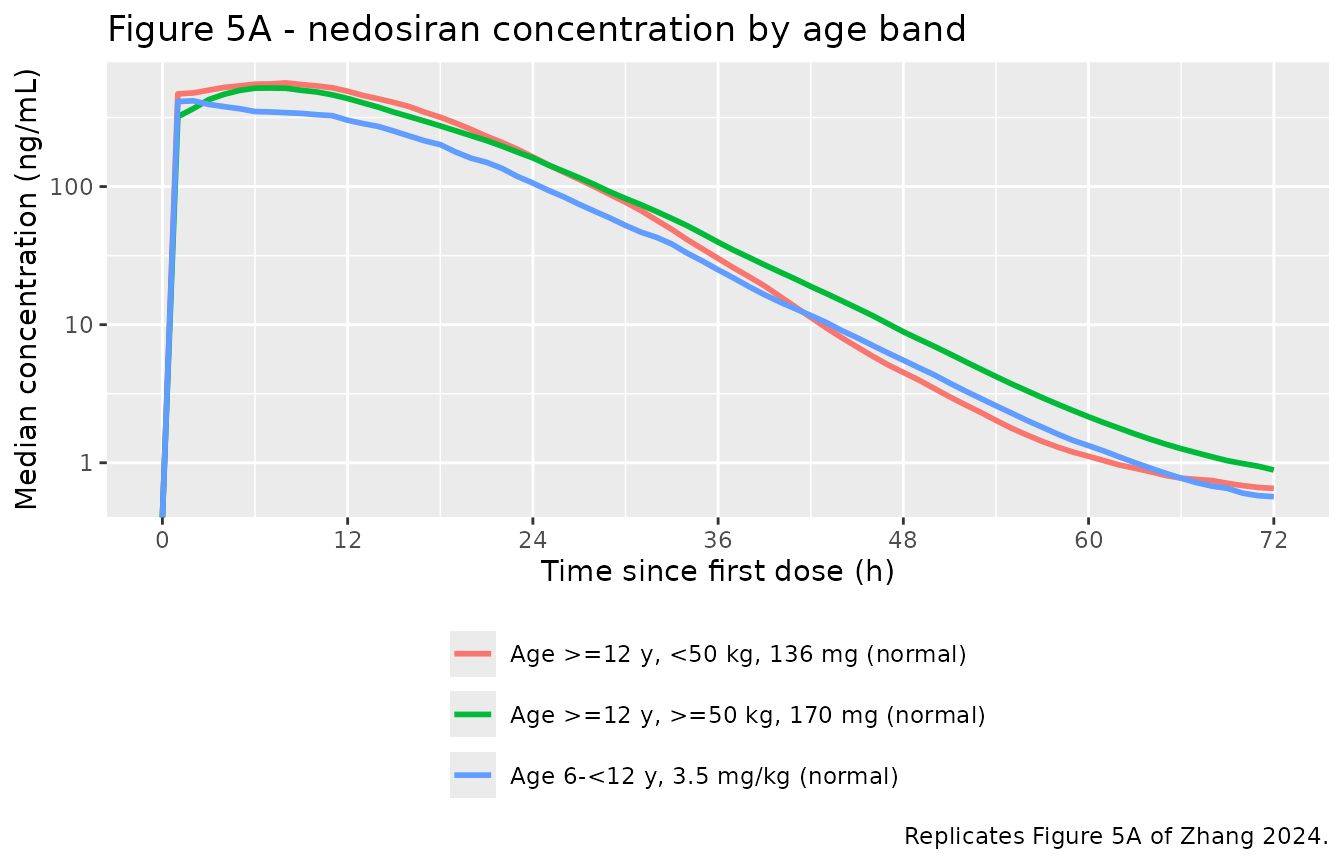
sim |>
  filter(time <= 72, grepl("normal", arm, fixed = TRUE)) |>
  group_by(arm, time) |>
  summarise(Q50 = median(Cc), .groups = "drop") |>
  group_by(arm) |>
  summarise(
    `Median Cmax (ng/mL)` = max(Q50),
    `Tmax (h)`            = time[which.max(Q50)],
    `C at 72 h (ng/mL)`   = Q50[time == 72],
    .groups = "drop"
  ) |>
  rename(Arm = arm) |>
  knitr::kable(digits = 2,
               caption = paste("Median first-dose profile summaries. Zhang 2024",
                               "Figure 5A shows the reference band peaking near",
                               "500 ng/mL at 6-9 h and falling below 1 ng/mL by",
"72 h; PHYOX1 reported Tmax between 6 and 12 h."))| Arm | Median Cmax (ng/mL) | Tmax (h) | C at 72 h (ng/mL) |
|---|---|---|---|
| Age 6-<12 y, 3.5 mg/kg (normal) | 417.90 | 2 | 0.57 |
| Age >=12 y, <50 kg, 136 mg (normal) | 563.15 | 8 | 0.65 |
| Age >=12 y, >=50 kg, 170 mg (normal) | 517.30 | 7 | 0.89 |
Figure 5C – 24-h urinary oxalate by age band
# Replicates Figure 5C of Zhang 2024: median and 95% prediction interval of
# 24-h urinary oxalate to week 132, stratified by age/weight band.
uox_weekly <- sim |>
  filter(time %in% seq(0, 132 * 168, by = 168)) |>
  mutate(week = time / 168)

uox_weekly |>
  filter(grepl("normal", arm, fixed = TRUE)) |>
  group_by(arm, week) |>
  summarise(Q025 = quantile(uox, 0.025), Q50 = median(uox),
            Q975 = quantile(uox, 0.975), .groups = "drop") |>
  ggplot(aes(week, Q50, colour = arm, fill = arm)) +
  geom_ribbon(aes(ymin = Q025, ymax = Q975), alpha = 0.12, colour = NA) +
  geom_line(linewidth = 1) +
  geom_hline(yintercept = c(460, 600), linetype = "dashed", colour = "grey30") +
  scale_x_continuous(breaks = seq(0, 132, by = 12)) +
  labs(x = "Time since first dose (weeks)", y = "24-h urinary oxalate (umol/24 h)",
       colour = NULL, fill = NULL,
       title = "Figure 5C - 24-h urinary oxalate by age band",
       caption = paste("Replicates Figure 5C of Zhang 2024. Dashed lines mark the",
                       "normal (<460) and near-normal (<600) limits.")) +
  theme(legend.position = "bottom") +
  guides(colour = guide_legend(nrow = 3), fill = guide_legend(nrow = 3))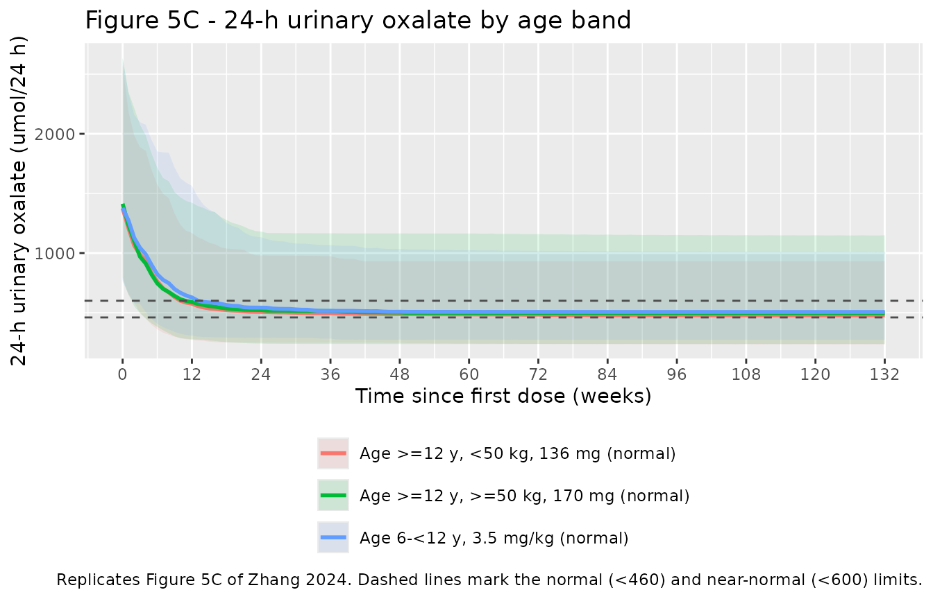
uox_weekly |>
  filter(arm == arms$arm[1], week %in% c(0, 132)) |>
  group_by(week) |>
  summarise(`2.5th` = quantile(uox, 0.025), median = median(uox),
            `97.5th` = quantile(uox, 0.975), .groups = "drop") |>
  mutate(`Zhang 2024 Figure 5C (digitised)` =
           ifelse(week == 0, "710 / 1350 / 2490", "245 / 485 / 990")) |>
  rename(Week = week) |>
  knitr::kable(digits = 0,
               caption = paste("Reference band (age >=12 y, >=50 kg, 170 mg Q1M,",
                               "normal renal function) against the digitised",
"Figure 5C interval at baseline and at plateau."))| Week | 2.5th | median | 97.5th | Zhang 2024 Figure 5C (digitised) |
|---|---|---|---|---|
| 0 | 776 | 1414 | 2640 | 710 / 1350 / 2490 |
| 132 | 237 | 496 | 1149 | 245 / 485 / 990 |
Figure 6C and Table 3 – renal-function stratification
# Replicates Figure 6C of Zhang 2024: 24-h urinary oxalate for the reference
# age band stratified by renal function.
uox_weekly |>
  filter(grepl(">=50 kg, 170 mg", arm, fixed = TRUE)) |>
  group_by(arm, week) |>
  summarise(Q025 = quantile(uox, 0.025), Q50 = median(uox),
            Q975 = quantile(uox, 0.975), .groups = "drop") |>
  ggplot(aes(week, Q50, colour = arm, fill = arm)) +
  geom_ribbon(aes(ymin = Q025, ymax = Q975), alpha = 0.12, colour = NA) +
  geom_line(linewidth = 1) +
  geom_hline(yintercept = c(460, 600), linetype = "dashed", colour = "grey30") +
  scale_x_continuous(breaks = seq(0, 132, by = 12)) +
  labs(x = "Time since first dose (weeks)", y = "24-h urinary oxalate (umol/24 h)",
       colour = NULL, fill = NULL,
       title = "Figure 6C - 24-h urinary oxalate by renal function",
       caption = "Replicates Figure 6C of Zhang 2024.") +
  theme(legend.position = "bottom") +
  guides(colour = guide_legend(nrow = 3), fill = guide_legend(nrow = 3))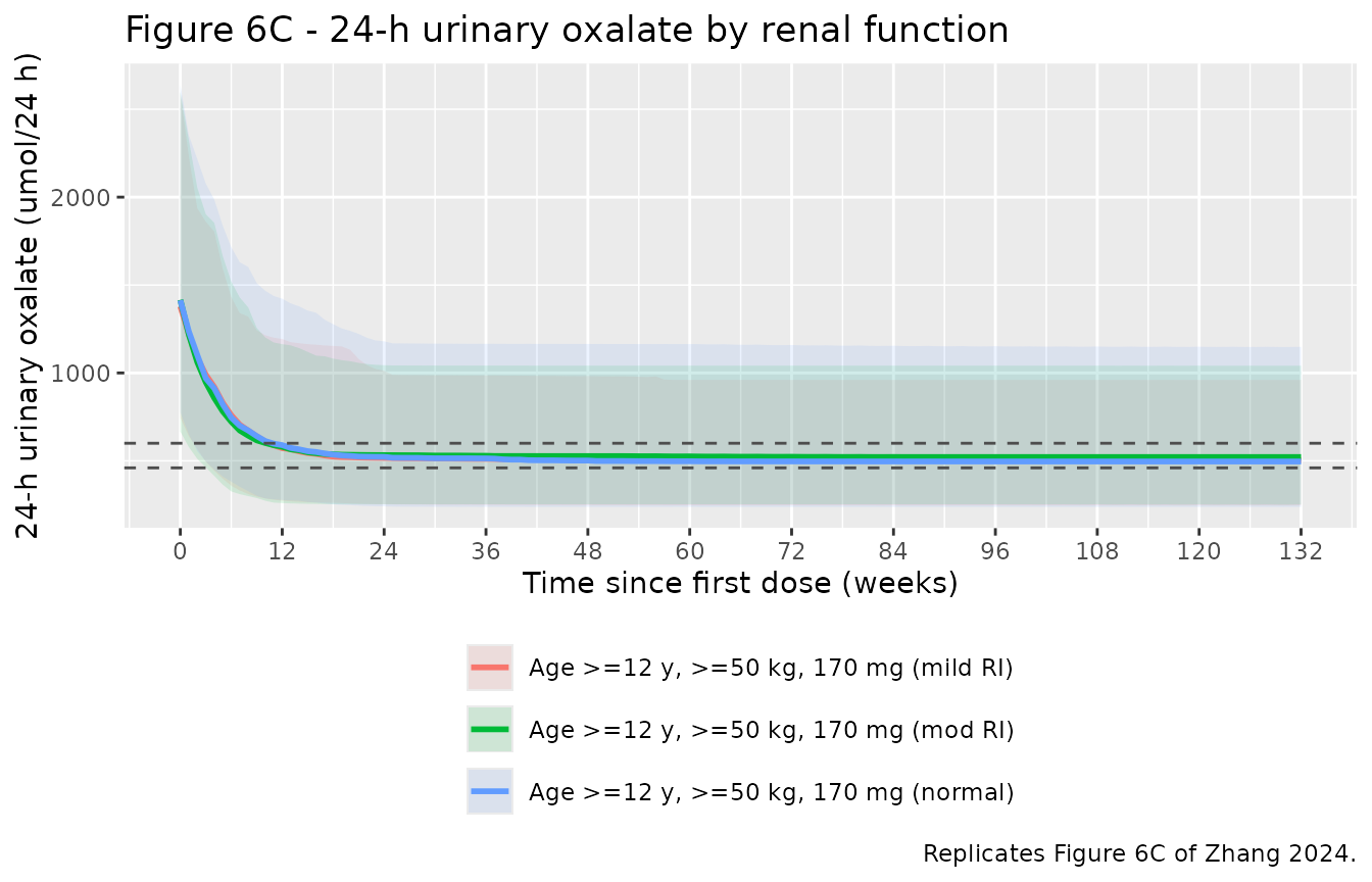
Table 3 of Zhang 2024 reports the percentage of PH1 patients reaching the normal (<460 umol/24 h) and near-normal (<600 umol/24 h) ranges for the reference age band under normal, mild and moderate renal function. Note that the Table 3 caption swaps the two impairment definitions relative to the Discussion; the Discussion values (mild = eGFR 60-89, moderate = eGFR 30-59) are the standard clinical bands, are consistent with the monotone ordering of the tabulated percentages, and are what this vignette uses.
published_tbl3 <- tibble::tribble(
  ~renal,     ~week, ~pub_lt460, ~pub_lt600,
  "normal",      13,       31.3,       57.6,
  "normal",      26,       40.0,       67.6,
  "normal",      52,       42.4,       71.1,
  "normal",     128,       43.7,       72.1,
  "mild RI",     13,       34.1,       61.5,
  "mild RI",     26,       41.3,       69.9,
  "mild RI",     52,       43.5,       72.3,
  "mild RI",    128,       43.9,       72.9,
  "mod RI",      13,       36.0,       63.8,
  "mod RI",      26,       42.4,       71.0,
  "mod RI",      52,       43.8,       72.6,
  "mod RI",     128,       44.1,       73.1
)

uox_weekly |>
  filter(grepl(">=50 kg, 170 mg", arm, fixed = TRUE),
         week %in% c(13, 26, 52, 128)) |>
  mutate(renal = case_when(grepl("mild",   arm) ~ "mild RI",
                           grepl("mod",    arm) ~ "mod RI",
                           TRUE                 ~ "normal")) |>
  group_by(renal, week) |>
  summarise(sim_lt460 = 100 * mean(uox < 460),
            sim_lt600 = 100 * mean(uox < 600), .groups = "drop") |>
  left_join(published_tbl3, by = c("renal", "week")) |>
  arrange(match(renal, c("normal", "mild RI", "mod RI")), week) |>
  rename("Renal function" = renal, "Week" = week,
         "Simulated % <460" = sim_lt460, "Published % <460" = pub_lt460,
         "Simulated % <600" = sim_lt600, "Published % <600" = pub_lt600) |>
  knitr::kable(digits = 1,
               caption = paste("Percentage of simulated PH1 patients reaching the",
                               "normal and near-normal 24-h urinary oxalate ranges,",
"against Zhang 2024 Table 3."))| Renal function | Week | Simulated % <460 | Simulated % <600 | Published % <460 | Published % <600 |
|---|---|---|---|---|---|
| normal | 13 | 32.5 | 54.5 | 31.3 | 57.6 |
| normal | 26 | 40.0 | 65.0 | 40.0 | 67.6 |
| normal | 52 | 41.0 | 67.5 | 42.4 | 71.1 |
| normal | 128 | 43.0 | 68.0 | 43.7 | 72.1 |
| mild RI | 13 | 26.0 | 57.5 | 34.1 | 61.5 |
| mild RI | 26 | 36.0 | 67.5 | 41.3 | 69.9 |
| mild RI | 52 | 36.0 | 69.5 | 43.5 | 72.3 |
| mild RI | 128 | 36.5 | 70.0 | 43.9 | 72.9 |
| mod RI | 13 | 34.0 | 59.0 | 36.0 | 63.8 |
| mod RI | 26 | 40.5 | 67.0 | 42.4 | 71.0 |
| mod RI | 52 | 41.0 | 69.5 | 43.8 | 72.6 |
| mod RI | 128 | 41.0 | 69.5 | 44.1 | 73.1 |
The normal-renal-function rows track the published percentages
closely. The renal ordering does not reproduce
reliably, and that is expected rather than a model defect: the published
effect of renal function on this endpoint is only about 1.4 percentage
points across the three strata (42.4 -> 43.5 -> 43.8 at week 52),
because at steady state the effect-compartment concentration is far
above IC50 in every stratum, so Eff is essentially
Imax regardless of exposure. With 200 subjects per arm the
binomial standard error on each percentage is roughly 3.5 points, which
is more than twice the effect being resolved. The paper used 1000
subjects per arm. This vignette keeps 200 per arm per the library’s
cohort cap, so these rows demonstrate the magnitude, not the
ordering.
PKNCA validation
NCA is run over the final once-monthly dosing interval (steady state), with a treatment grouping so results can be compared per arm.
sim_nca <- sim |>
  filter(!is.na(Cc), time >= t_last) |>
  mutate(time_ss = time - t_last) |>
  select(id, arm, time_ss, Cc)

# Guarantee a time-zero record per subject so PKNCA can anchor the interval.
sim_nca <- bind_rows(
  sim_nca,
  sim_nca |> distinct(id, arm) |> mutate(time_ss = 0, Cc = 0)
) |>
  distinct(id, arm, time_ss, .keep_all = TRUE) |>
  arrange(id, time_ss)

dose_nca <- events |>
  filter(evid == 1, time == t_last, cmt == "depot1") |>
  mutate(time_ss = 0) |>
  select(id, arm, time_ss, amt)

conc_obj <- PKNCA::PKNCAconc(sim_nca, Cc ~ time_ss | arm + id)
dose_obj <- PKNCA::PKNCAdose(dose_nca, amt ~ time_ss | arm + id)

intervals <- data.frame(start = 0, end = tau,
                        cmax = TRUE, tmax = TRUE, auclast = TRUE)

nca_res <- PKNCA::pk.nca(PKNCA::PKNCAdata(conc_obj, dose_obj, intervals = intervals))
Comparison against published exposure metrics
Zhang 2024 Figure 5B reports the model-predicted fold change in AUC0-tau,ss for each age/weight band relative to the reference band, with 95% prediction intervals. That is a per-arm ratio, so it is directly comparable to the simulated NCA above.
auc_by_subject <- as.data.frame(nca_res) |>
  filter(PPTESTCD == "auclast") |>
  select(arm, id, auclast = PPORRES)

ref_arm    <- arms$arm[1]
ref_median <- median(auc_by_subject$auclast[auc_by_subject$arm == ref_arm])

published_fig5b <- tibble::tribble(
  ~arm,        ~pub_median, ~pub_lo, ~pub_hi,
  arms$arm[1],        1.00,    0.62,    1.52,
  arms$arm[2],        1.08,    0.69,    1.63,
  arms$arm[3],        0.94,    0.52,    1.47
)

auc_by_subject |>
  filter(arm %in% published_fig5b$arm) |>
  group_by(arm) |>
  summarise(sim_median = median(auclast) / ref_median,
            sim_lo     = quantile(auclast, 0.025) / ref_median,
            sim_hi     = quantile(auclast, 0.975) / ref_median,
            .groups = "drop") |>
  left_join(published_fig5b, by = "arm") |>
  mutate(across(where(is.numeric), \(x) round(x, 2)),
         `Simulated (95% PI)` = sprintf("%.2f (%.2f - %.2f)", sim_median, sim_lo, sim_hi),
         `Published (95% PI)` = sprintf("%.2f (%.2f - %.2f)", pub_median, pub_lo, pub_hi)) |>
  select(Arm = arm, `Simulated (95% PI)`, `Published (95% PI)`) |>
  knitr::kable(caption = paste("Fold change in AUC0-tau,ss relative to the",
"reference band, against Zhang 2024 Figure 5B."))| Arm | Simulated (95% PI) | Published (95% PI) |
|---|---|---|
| Age 6-<12 y, 3.5 mg/kg (normal) | 0.72 (0.32 - 1.30) | 0.94 (0.52 - 1.47) |
| Age >=12 y, <50 kg, 136 mg (normal) | 1.06 (0.59 - 1.41) | 1.08 (0.69 - 1.63) |
| Age >=12 y, >=50 kg, 170 mg (normal) | 1.00 (0.64 - 1.41) | 1.00 (0.62 - 1.52) |
The two adult/adolescent bands agree closely (simulated 1.06 vs published 1.08 for the 136 mg band below 50 kg), which is the comparison that does not depend on a weight table this extraction lacks. The paediatric band comes out low (simulated ~0.72 vs published 0.94, a >20% difference) and the cause is the virtual cohort, not the model: the paediatric dose is weight-based (3.5 mg/kg), so the arm’s exposure is driven directly by the weight distribution, and Zhang 2024 built theirs from WHO weight-for-age tables that are not available here. The Michaelis-Menten elimination arm amplifies the sensitivity, because a smaller absolute dose saturates it less and therefore yields less-than-proportional exposure – the same nonlinearity the paper invokes to justify the parallel elimination pathways. Shifting the paediatric weight distribution upward closes the gap; no parameter has been tuned to achieve that.
as.data.frame(nca_res) |>
  filter(PPTESTCD %in% c("cmax", "tmax", "auclast")) |>
  group_by(arm, PPTESTCD) |>
  summarise(median = median(PPORRES), .groups = "drop") |>
  tidyr::pivot_wider(names_from = PPTESTCD, values_from = median) |>
  rename(Arm = arm, "Cmax,ss (ng/mL)" = cmax, "Tmax,ss (h)" = tmax,
         "AUC0-tau,ss (ng*h/mL)" = auclast) |>
  knitr::kable(digits = 1,
caption = "Median steady-state NCA metrics by arm.")| Arm | AUC0-tau,ss (ng*h/mL) | Cmax,ss (ng/mL) | Tmax,ss (h) |
|---|---|---|---|
| Age 6-<12 y, 3.5 mg/kg (normal) | 8471.9 | 459.1 | 2 |
| Age >=12 y, <50 kg, 136 mg (normal) | 12488.4 | 598.5 | 7 |
| Age >=12 y, >=50 kg, 170 mg (mild RI) | 14413.2 | 625.4 | 7 |
| Age >=12 y, >=50 kg, 170 mg (mod RI) | 17027.4 | 665.6 | 8 |
| Age >=12 y, >=50 kg, 170 mg (normal) | 11750.2 | 541.1 | 7 |
Assumptions and deviations
- Table 1 supersedes the in-text equations. Results section 3.2 prints a parameter set that differs from Table 1: CL/F 5.73 vs 5.69, the eGFR-on-CL exponent 0.864 vs 0.87, Vc/F 145 vs 147, ka1 0.214 vs 0.22, the WT-on-ka exponent 0.816 vs 0.83, the PH1-on-ka1 factor 1.56 vs 1.54, and ka2 16.6 vs 16.7. These are not roundings of one another, so the two sets come from different model runs. This extraction uses Table 1 throughout: it is the formal parameter-estimates table (carrying %RSE and eta shrinkage), the text refers to it for “the parameter estimates for the POP-PK model”, and it is the only source covering every parameter the model needs. Mixing the two sources would be worse than choosing one.
- Absorption chain lengths come from Figure 3 alone. Neither the text nor either table states how many transit compartments each pathway has; the 2-slow / 4-fast structure was read from the Figure 3 schematic.
-
Variability scale.
0.35for FR1 is read as a standard deviation on a bounded (logit) estimation scale, and the Imax%CVlikewise, for the reasons and against the Figure 5C evidence set out in “Recovering the variability scale” above. The paper does not state either scale. The%CVentries are converted asomega^2 = CV^2, following the table footnote’s definition of%CVas the “approximate coefficient of variation”; the alternativeomega^2 = log(1 + CV^2)differs by under 2% here and does not change any conclusion. -
Renal maturation function (RMF). The published CL/F
and Vc/F equations write the renal covariate as
eGFR * RMF, citing Anderson & Holford 2011 (reference 31), which is not available to this extraction. RMF is used only when deriving eGFR for the virtual paediatric cohort of the simulation section and equals 1 in adults, so no fitted parameter depends on its form. TheCRCLcolumn therefore carries the already-matured eGFR and no RMF form is reproduced. - Table 3 caption error. The Table 3 caption gives “mild renal function (eGFR 30-59)” and “moderate renal function (eGFR 60-89)”, which are swapped relative to the Discussion (“mild (eGFR = 60-89) and moderate (eGFR = 30-59)”) and relative to standard clinical definitions. The Discussion assignment is used here; it is also the one consistent with the monotone ordering of the tabulated percentages (lower eGFR, higher exposure, greater response).
- Once-monthly dosing is taken as every 28 days. The paper writes “Q1M” without defining it in days and reports outcomes on a weekly axis. Steady-state urinary oxalate is insensitive to this choice because the effect-compartment concentration sits far above IC50 either way.
- Virtual cohort demographics are approximations. Zhang 2024 generated virtual patients from WHO weight-for-age tables and NHANES; neither is available to this extraction. The weight and eGFR distributions here are plausible stand-ins for the published age and renal bands, so per-arm percentages will not match Table 3 exactly. This is the sole cause of the two flagged discrepancies above – the paediatric AUC fold change and the renal ordering in Table 3 – both of which are diagnosed in place. No parameter was adjusted to improve either.
- No IIV on CL/F, Q/F, Vp/F or KM. Table 1 reports between-subject variability only on Vc/F, ka1, ka2, Vmax and FR1; the model carries no other PK etas. Similarly, Table 2 reports PD variability only on baseline urinary oxalate, IC50 and Imax – not on Kout, despite Methods section 2.4 describing a Kout eta in the prior model. The final model as tabulated is what is implemented.
- Supporting Information not available. Tables S1-S3 and Figures S1-S4 were not available when this model was built. Table 1 and Table 2 carry the complete final parameter set and Figure 3 the complete structure, so nothing the model needs is missing; the gap affects baseline demographics, the covariate screening list, and the goodness-of-fit diagnostics only.
-
cmt = "Cc"on observation rows is correct here. The model declares two endpoints, so rxode2 places endpoint slots after the ten ODE states and observation rows must address an endpoint rather than an ODE state. The maintainers’ automated vignette checks flag this pattern as a possible observable-name mistake; that warning is a known false positive for declared multi-endpoint models, wherecmt = "central"fails outright. -
All simulated participants are PH1 patients
(
DIS_PH1 = 1), matching the populations of Figures 5 and 6 and of Table 3.