Piperaquine PK and QTc (Wattanakul 2020)
Source:vignettes/articles/Wattanakul_2020_piperaquine.Rmd
Wattanakul_2020_piperaquine.RmdModel and source
- Citation: Wattanakul T, Ogutu B, Kabanywanyi AM, et al., Tarning J. (2020). Pooled multicenter analysis of cardiovascular safety and population pharmacokinetic properties of piperaquine in African patients with uncomplicated falciparum malaria. Antimicrobial Agents and Chemotherapy 64(7):e01848-19. doi:10.1128/AAC.01848-19 (PMC7318010).
- Article: https://doi.org/10.1128/AAC.01848-19
- Supplement: AAC.01848-19-s0001.pdf (supplementary Equations 1-2, Tables S1-S3).
The paper builds its models sequentially, and the package ships them as three files:
| Model | What it describes | Source |
|---|---|---|
Wattanakul_2020_piperaquine |
Population PK of piperaquine (the Hoglund 2017 meta-analysis model refitted with a frequentist prior) | Table 2 |
Wattanakul_2020_piperaquine_qtc |
Sigmoid Emax model of the absolute QTcSSB interval, PK embedded | Table 4, Equation 9 |
Wattanakul_2020_piperaquine_dqtc |
Sigmoid Emax model of the change from baseline in QTcSSB, PK embedded | Table S2, supplementary Equation 2 |
QTcSSB is the QT interval corrected with a study-specific exponent, QTc = QT / RR^0.476. The exponent was estimated by regressing log QT on log RR across the pre-treatment ECGs (Results, ‘QT interval correction methods’). The PD models were fitted to individually predicted piperaquine concentrations, so each PD file embeds the PK model and has concentration as a latent driver.
mod_pk <- rxode2::rxode2(readModelDb("Wattanakul_2020_piperaquine"))
#> Warning: some etas defaulted to non-mu referenced, possible parsing error: etaiov_fdepot_1, etaiov_fdepot_2, etaiov_fdepot_3, etaiov_mtt_1, etaiov_mtt_2, etaiov_mtt_3
#> as a work-around try putting the mu-referenced expression on a simple line
mod_qtc <- rxode2::rxode2(readModelDb("Wattanakul_2020_piperaquine_qtc"))
#> Warning: some etas defaulted to non-mu referenced, possible parsing error: etaiov_fdepot_1, etaiov_fdepot_2, etaiov_fdepot_3, etaiov_mtt_1, etaiov_mtt_2, etaiov_mtt_3
#> as a work-around try putting the mu-referenced expression on a simple line
mod_dqtc <- rxode2::rxode2(readModelDb("Wattanakul_2020_piperaquine_dqtc"))
#> Warning: some etas defaulted to non-mu referenced, possible parsing error: etaiov_fdepot_1, etaiov_fdepot_2, etaiov_fdepot_3, etaiov_mtt_1, etaiov_mtt_2, etaiov_mtt_3
#> as a work-around try putting the mu-referenced expression on a simple line
Population
The analysis used 1,000 patients with uncomplicated P.
falciparum malaria from the nested PK-ECG cohort of a
post-licensing pharmacovigilance study of dihydroartemisinin-piperaquine
(Eurartesim; NCT02199951). Patients came from 10 sites: Burkina Faso (n
= 299), Ghana (n = 442), Mozambique (n = 89) and Tanzania (n = 170).
They were mostly children. By age, 0.6% were under 1 year, 23.8% were 1
to < 5 years, 45.0% were 5 to < 12 years, 12.7% were 12 to < 18
years and 17.9% were adults. Median age was 7.5 years (IQR 5-12), median
weight 21 kg (IQR 15-38), and 51.8% were female (Table 1). Patients
received weight-banded doses once daily for 3 days under direct
observation. The PK dataset comprised 2,989 plasma samples taken at
about 0, 48, 52, 120, 144 and 168 h after the first dose. ECGs were
recorded before the first dose, before and after the day-3 dose, and on
day 7. The same information is available programmatically via
readModelDb("Wattanakul_2020_piperaquine")()$population.
Source trace
Per-parameter source locations are recorded inline next to each
ini() entry in the three model files. They are collected
here for review.
| Equation / parameter | Value | Source location |
|---|---|---|
lmtt (MTT) |
2.13 h | Table 2 |
lcl (CL/F at 54 kg, fully mature) |
53.1 L/h | Table 2 |
lvc (Vc/F) |
1,730 L | Table 2 |
lq (Q1/F) |
282 L/h | Table 2 |
lvp (Vp1/F) |
3,290 L | Table 2 |
lq2 (Q2/F) |
82.9 L/h | Table 2 |
lvp2 (Vp2/F) |
25,100 L | Table 2 |
lfdepot (F) |
1, fixed | Table 2 |
e_doseocc_f |
0.237, fixed | Table 2 ‘Dose occasion effect on F’ |
mat_mf50, mat_hill
|
0.575 y, 5.51, fixed | Table 2; Equation 3 |
e_wt_cl, e_wt_vc
|
0.75, 1, fixed; reference 54 kg | Methods; Table 2 footnote b |
| IIV F, MTT, Vc, Vp1, Q2, Vp2 | 38.2, 37.5, 90.5, 23.4, 27.1, 31.8 %CV | Table 2; omega^2 = log(CV^2 + 1) (footnote b) |
| IOV F, MTT | 42.8, 44.7 %CV | Table 2; Equation 2 |
propSd |
sqrt(0.198) | Table 2 sigma (variance of the log-scale additive error) |
| Two transits with ka = ktr, three-compartment disposition | – | Results ‘Population pharmacokinetic modeling’; Methods |
QTc: e0
|
421 ms | Table 4 QTcBaseline |
QTc: lemax
|
35 ms | Table 4 |
QTc: lec50
|
209 ng/mL | Table 4 |
QTc: lhill
|
1.69 | Table 4 gamma |
QTc: e_age_ec50
|
0.0410 per year | Table 4 ‘Effect of age on EC50 (%)’ = 4.10 |
QTc: etae0
|
17.0 ms SD (additive) | Table 4, footnote d |
QTc: etalemax, etalec50
|
49.1, 119.3 %CV | Table 4, footnote e |
QTc: addSd
|
11.6 ms | Table 4 sigma |
QTc equation
(QTcBaseline + eta) + Emax * Cp^gamma / (Cp^gamma + EC50^gamma)
|
– | Equation 9 |
dQTc: e0
|
0, fixed | Table S2 |
dQTc: lemax, lec50,
lhill
|
47.5 ms, 319 ng/mL, 1.22 | Table S2 |
dQTc: e_age_ec50
|
0.0287 per year | Table S2 ‘Effect of age on EC50 (%)’ = 2.87 |
dQTc: etae0
|
10.6 ms SD (additive) | Table S2, footnote c |
dQTc: etalemax, etalec50
|
29.6, 217 %CV | Table S2, footnote d |
dQTc: addSd
|
12.6 ms | Table S2 sigma |
| dQTc equation | – | Supplementary Equation 2 |
Age effect EC50 * (1 + e_age_ec50 * (AGE - 7.5))
|
– | Functional form not printed; the maintainers’ reading (see Assumptions) |
Virtual cohorts
Two cohorts are used, each capped at 200 simulated patients per arm.
- A study-like cohort follows the Table 1 age mix, with body weight derived from age. It receives the regimen used in the study: the Table 5 ‘old’ WHO weight bands, three daily doses. It is used for the Figure 1 VPC, for PKNCA and for the Table S3 categorical comparison.
- Simulation-scenario cohorts reproduce the paper’s Monte Carlo design: body weight uniform over 5-100 kg, age assigned from weight, and four arms (old or new regimen, acute or mass drug administration). They are used to compare against the reported QTcmax and DeltaQTcmax.
The paper does not publish its age-weight relationship. The maintainers use an approximate median weight-for-age curve for African children, running from 7 kg at 6 months to 56 kg at 25 years. Doses are converted from piperaquine phosphate to piperaquine base with the 57.7% factor used by the Hoglund 2017 prior model.
set.seed(20200623L)

# Approximate median weight-for-age (maintainers' assumption; see Assumptions).
age_knots <- c(0.5, 1, 2, 3, 4, 5, 6, 7, 8, 9, 10, 12, 14, 16, 18, 25)
wt_knots <- 0.9 * c(7.6, 9.6, 12.2, 14.3, 16.3, 18.3, 20.5, 22.9, 25.5, 28.5, 32, 40, 50, 56, 59, 62)
wt_from_age <- function(age) stats::approx(age_knots, wt_knots, xout = pmin(age, 25), rule = 2)$y
age_from_wt <- function(wt) stats::approx(wt_knots, age_knots, xout = wt, rule = 2)$y

# Table 5 piperaquine phosphate dose (mg) per daily dose.
dose_old <- function(wt) {
  dplyr::case_when(wt < 13 ~ 160, wt < 24 ~ 320, wt < 36 ~ 640, wt < 75 ~ 960, TRUE ~ 1280)
}
dose_new <- function(wt) {
  dplyr::case_when(
    wt < 8 ~ 160, wt < 11 ~ 240, wt < 17 ~ 320, wt < 25 ~ 480,
    wt < 36 ~ 640, wt < 60 ~ 960, wt < 80 ~ 1280, TRUE ~ 1600
  )
}
base_fraction <- 0.577

# Study-like cohort: Table 1 age groups; ages within 5-12 y are skewed
# towards the younger end so the cohort median age is close to 7.5 y.
n_study <- 200L
grp <- sample(1:5, n_study, replace = TRUE, prob = c(0.6, 23.8, 45.0, 12.7, 17.9))
u <- runif(n_study)
age <- dplyr::case_when(
  grp == 1 ~ 0.5 + 0.5 * u,
  grp == 2 ~ 1 + 4 * u,
  grp == 3 ~ 5 + 7 * u^2,
  grp == 4 ~ 12 + 6 * u,
  TRUE ~ 18 + 32 * u
)
study <- data.frame(
  id = seq_len(n_study),
  AGE = age,
  WT = pmax(5, wt_from_age(age) * exp(rnorm(n_study, 0, 0.12)))
) |>
  dplyr::mutate(pqp_mg = dose_old(WT), arm = "study cohort")

knitr::kable(
  data.frame(
    Statistic = c("Median age (y)", "Median weight (kg)"),
    Simulated = c(round(median(study$AGE), 1), round(median(study$WT), 1)),
    `Table 1` = c("7.5 (IQR 5-12)", "21 (IQR 15-38)"),
    check.names = FALSE
  ),
  caption = "Study-like virtual cohort against Table 1."
)| Statistic | Simulated | Table 1 |
|---|---|---|
| Median age (y) | 6.9 | 7.5 (IQR 5-12) |
| Median weight (kg) | 19.3 | 21 (IQR 15-38) |
The event builder places one dose per day. Each dose row carries
OCC = 1, 2, 3 within a course, and every observation row
carries the OCC of the most recent dose. Observation rows
sit on the central state; Cc,
QTcS and the other observables are computed at those
rows.
build_events <- function(subj, dose_times, occ, obs_times, id_offset = 0L) {
  out <- lapply(seq_len(nrow(subj)), function(i) {
    s <- subj[i, ]
    d <- data.frame(time = dose_times, evid = 1L, amt = s$pqp_mg * base_fraction, cmt = "depot", OCC = occ)
    o <- data.frame(
      time = obs_times, evid = 0L, amt = 0, cmt = "central",
      OCC = occ[pmax(1L, findInterval(obs_times, dose_times))]
    )
    x <- rbind(d, o)
    x$id <- s$id + id_offset
    x$WT <- s$WT
    x$AGE <- s$AGE
    x$arm <- s$arm
    x
  })
  ev <- dplyr::bind_rows(out)
  ev[order(ev$id, ev$time, -ev$evid), ]
}

acute_doses <- c(0, 24, 48)
obs_study <- sort(unique(c(seq(0, 72, by = 1), seq(76, 168, by = 4))))
ev_study <- build_events(study, acute_doses, 1:3, obs_study)
stopifnot(!anyDuplicated(ev_study[, c("id", "time", "evid")]))
Simulation
rxode2::rxSetSeed(20200623L)
sim_pk <- rxode2::rxSolve(mod_pk, events = ev_study, keep = c("WT", "AGE", "arm")) |>
  as.data.frame()
Replicate published figures
Figure 1: PK visual predictive check
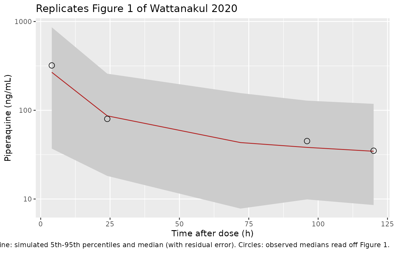
Figure 1 plots the observed piperaquine concentrations against time after the most recent dose. The sampling times, relative to the first dose, map onto time after dose as follows: 48 h is the pre-dose day-3 sample (24 h after the second dose), 52 h is about 4 h after the third dose, and 120, 144 and 168 h are 72, 96 and 120 h after the last dose. The observed medians in the table below were read off Figure 1 by the maintainers. They are approximate to within about 10%.
tad_map <- data.frame(time = c(48, 52, 120, 144, 168), tad = c(24, 4, 72, 96, 120))
fig1 <- sim_pk |>
  dplyr::inner_join(tad_map, by = "time") |>
  dplyr::group_by(tad) |>
  dplyr::summarise(
    p05 = quantile(sim, 0.05), p50 = quantile(sim, 0.50), p95 = quantile(sim, 0.95),
    ipred_p50 = median(ipredSim), .groups = "drop"
  )
# Observed medians digitised from Figure 1 (red solid line).
fig1_obs <- data.frame(tad = c(4, 24, 96, 120), obs_p50 = c(320, 80, 45, 35))

ggplot(fig1, aes(tad)) +
  geom_ribbon(aes(ymin = p05, ymax = p95), fill = "grey80") +
  geom_line(aes(y = p50), colour = "firebrick") +
  geom_point(data = fig1_obs, aes(y = obs_p50), shape = 1, size = 3) +
  scale_y_log10() +
  labs(
    x = "Time after dose (h)", y = "Piperaquine (ng/mL)",
    title = "Replicates Figure 1 of Wattanakul 2020",
    caption = "Band and line: simulated 5th-95th percentiles and median (with residual error). Circles: observed medians read off Figure 1."
  )
vpc_cmp <- fig1 |>
  dplyr::inner_join(fig1_obs, by = "tad") |>
  dplyr::mutate(ratio = p50 / obs_p50)
knitr::kable(
  vpc_cmp |>
    dplyr::select(tad, p50, obs_p50, ratio) |>
    dplyr::rename(
      "Time after dose (h)" = tad, "Simulated median (ng/mL)" = p50,
      "Figure 1 observed median (ng/mL)" = obs_p50, "Ratio" = ratio
    ),
  digits = 2, caption = "Simulated versus observed median piperaquine concentration."
)| Time after dose (h) | Simulated median (ng/mL) | Figure 1 observed median (ng/mL) | Ratio |
|---|---|---|---|
| 4 | 267.96 | 320 | 0.84 |
| 24 | 86.54 | 80 | 1.08 |
| 96 | 38.18 | 45 | 0.85 |
| 120 | 34.54 | 35 | 0.99 |
PKNCA validation
NCA is run over the three-dose course and the 5 days that follow (0-168 h), grouped by the Table 5 weight band.
sim_nca <- sim_pk |>
  dplyr::filter(!is.na(Cc)) |>
  dplyr::mutate(band = cut(WT, c(0, 13, 24, 36, 75, Inf), right = FALSE,
                           labels = c("5-12 kg", "13-23 kg", "24-35 kg", "36-74 kg", ">=75 kg"))) |>
  dplyr::select(id, time, Cc, band)
sim_nca <- dplyr::bind_rows(
  sim_nca,
  sim_nca |> dplyr::distinct(id, band) |> dplyr::mutate(time = 0, Cc = 0)
) |>
  dplyr::distinct(id, band, time, .keep_all = TRUE) |>
  dplyr::arrange(id, band, time)

dose_df <- ev_study |>
  dplyr::filter(evid == 1) |>
  dplyr::select(id, time, amt) |>
  dplyr::inner_join(dplyr::distinct(sim_nca, id, band), by = "id")

conc_obj <- PKNCA::PKNCAconc(sim_nca, Cc ~ time | band + id, concu = "ng/mL", timeu = "h")
dose_obj <- PKNCA::PKNCAdose(dose_df, amt ~ time | band + id, doseu = "mg")
intervals <- data.frame(start = 0, end = 168, cmax = TRUE, tmax = TRUE, auclast = TRUE)
nca_res <- PKNCA::pk.nca(PKNCA::PKNCAdata(conc_obj, dose_obj, intervals = intervals))
knitr::kable(summary(nca_res), caption = "Simulated NCA by weight band, 0-168 h (study-like cohort).")| Interval Start | Interval End | band | N | AUClast (h*ng/mL) | Cmax (ng/mL) | Tmax (h) |
|---|---|---|---|---|---|---|
| 0 | 168 | 5-12 kg | 28 | 11400 [54.3] | 270 [68.8] | 50.0 [2.00, 55.0] |
| 0 | 168 | 13-23 kg | 90 | 14700 [56.3] | 347 [79.2] | 50.0 [1.00, 60.0] |
| 0 | 168 | 24-35 kg | 24 | 21700 [50.5] | 516 [82.7] | 51.0 [3.00, 54.0] |
| 0 | 168 | 36-74 kg | 58 | 17400 [45.8] | 372 [73.6] | 51.0 [1.00, 57.0] |
Table 3 of the paper reports a median piperaquine Cmax per QTc stratum, and the paper does not say how Cmax was derived. The DeltaQTcSSB <= 30 ms stratum holds 64% of patients and has a median Cmax of 694 ng/mL. The comparison below sets the whole simulated cohort against that stratum.
nca_all <- PKNCA::pk.nca(PKNCA::PKNCAdata(
  PKNCA::PKNCAconc(dplyr::mutate(sim_nca, grp = "all"), Cc ~ time | grp + id, concu = "ng/mL", timeu = "h"),
  PKNCA::PKNCAdose(dplyr::mutate(dose_df, grp = "all"), amt ~ time | grp + id, doseu = "mg"),
  intervals = data.frame(start = 0, end = 168, cmax = TRUE)
))
cmp <- nlmixr2lib::ncaComparisonTable(
  simulated = nca_all,
  reference = tibble::tibble(grp = "all", cmax = 694),
  by = "grp",
  units = c(cmax = "ng/mL"),
  tolerance_pct = 20
)
knitr::kable(cmp, caption = "Simulated Cmax against the Table 3 median. * differs by more than 20%.")| NCA parameter | grp | Reference | Simulated | % diff |
|---|---|---|---|---|
| Cmax (ng/mL) | all | 694 | 342 | -50.7%* |
The simulated median Cmax is about half the Table 3 value, which is starred. The Figure 1 VPC shows that this is not a scale error in the model. The observed median about 4 h after the third dose is roughly 320 ng/mL, and the simulation reproduces it. The Table 3 number therefore cannot be a median of those same concentrations. It is probably a per-patient maximum derived some other way that the paper does not describe, so the discrepancy is recorded here and not used as a gate.
QTc simulations
Study cohort: Table S3 categorical distribution
The paper’s Table S3 simulates the study population from the final DeltaQTc model and reports the maximum change from baseline in QTcSSB in three bands: <= 30 ms (65.8%), 31-60 ms (29.8%) and > 60 ms (4.35%). In the simulation below, each patient’s maximum is taken over the post-treatment ECG times (pre-dose day 3, about 4 h after the day-3 dose, and day 7). Residual error is included, as it would be in an observed ECG.
ecg_times <- c(48, 52, 144)
rxode2::rxSetSeed(20200624L)
sim_d <- rxode2::rxSolve(mod_dqtc, events = ev_study, keep = c("WT", "AGE")) |>
  as.data.frame()
s3 <- sim_d |>
  dplyr::filter(time %in% ecg_times) |>
  dplyr::group_by(id) |>
  dplyr::summarise(dmax = max(sim), .groups = "drop") |>
  dplyr::mutate(band = cut(dmax, c(-Inf, 30, 60, Inf), labels = c("<=30 ms", "31-60 ms", ">60 ms")))
s3_tab <- s3 |>
  dplyr::count(band, .drop = FALSE) |>
  dplyr::mutate(pct = 100 * n / sum(n), published = c(65.8, 29.8, 4.35))
knitr::kable(
  s3_tab |> dplyr::rename("DeltaQTcSSB max" = band, "Simulated n" = n, "Simulated (%)" = pct, "Table S3 (%)" = published),
  digits = 1, caption = "Maximum DeltaQTcSSB category, study-like cohort (n = 200)."
)| DeltaQTcSSB max | Simulated n | Simulated (%) | Table S3 (%) |
|---|---|---|---|
| <=30 ms | 120 | 60.0 | 65.8 |
| 31-60 ms | 63 | 31.5 | 29.8 |
| >60 ms | 17 | 8.5 | 4.3 |
Simulation scenarios: acute treatment and mass drug administration
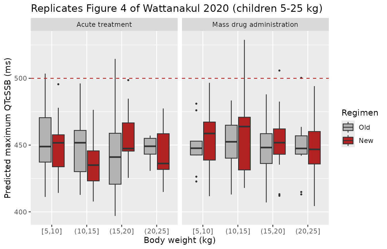
The paper simulates two settings. Acute treatment is a single three-day course. Mass drug administration (MDA) is the three-day course repeated monthly for three months. Each setting is simulated under the old and the new WHO regimen (Table 5). The absolute-QTc model is used, and predicted maxima exclude residual error. With residual error included, the lower 2.5th percentile of DeltaQTcmax could not stay positive as the published 2.31-2.90 ms does. Each arm holds 200 simulated patients with body weight uniform over 5-100 kg.
n_arm <- 200L
make_arm <- function(arm, dose_fun) {
  wt <- runif(n_arm, 5, 100)
  data.frame(id = seq_len(n_arm), WT = wt, AGE = age_from_wt(wt), pqp_mg = dose_fun(wt), arm = arm)
}
mda_doses <- c(acute_doses, acute_doses + 720, acute_doses + 1440)
obs_acute <- seq(0, 96, by = 1)
obs_mda <- sort(unique(c(obs_acute, obs_acute + 720, obs_acute + 1440)))
ev_scen <- dplyr::bind_rows(
  build_events(make_arm("Acute, old regimen", dose_old), acute_doses, 1:3, obs_acute, 0L),
  build_events(make_arm("Acute, new regimen", dose_new), acute_doses, 1:3, obs_acute, 200L),
  build_events(make_arm("MDA, old regimen", dose_old), mda_doses, rep(1:3, 3), obs_mda, 400L),
  build_events(make_arm("MDA, new regimen", dose_new), mda_doses, rep(1:3, 3), obs_mda, 600L)
)
stopifnot(!anyDuplicated(ev_scen[, c("id", "time", "evid")]))

rxode2::rxSetSeed(20200625L)
sim_q <- rxode2::rxSolve(mod_qtc, events = ev_scen, keep = c("WT", "AGE", "arm")) |>
  as.data.frame()

qmax <- sim_q |>
  dplyr::group_by(arm, id) |>
  dplyr::summarise(
    qtcmax = max(ipredSim),
    dqtcmax = max(ipredSim) - ipredSim[time == 0][1],
    WT = WT[1], .groups = "drop"
  )
scen <- qmax |>
  dplyr::group_by(arm) |>
  dplyr::summarise(
    qtc_med = median(qtcmax), qtc_lo = quantile(qtcmax, 0.025), qtc_hi = quantile(qtcmax, 0.975),
    dq_med = median(dqtcmax), dq_lo = quantile(dqtcmax, 0.025), dq_hi = quantile(dqtcmax, 0.975),
    pct_500 = 100 * mean(qtcmax > 500), pct_d60 = 100 * mean(dqtcmax > 60), .groups = "drop"
  )
published <- data.frame(
  arm = c("Acute, old regimen", "Acute, new regimen", "MDA, old regimen", "MDA, new regimen"),
  pub_qtc = c("440 (401-489)", "441 (401-490)", "440 (401-490)", "441 (402-491)"),
  pub_qtc_med = c(440, 441, 440, 441),
  pub_dq = c("16.8 (2.31-56.9)", "18.0 (2.67-58.6)", "17.6 (2.58-57.9)", "18.5 (2.90-59.3)"),
  pub_dq_med = c(16.8, 18.0, 17.6, 18.5),
  pub_500 = c(1.1, 1.2, 1.2, 1.3)
)
scen_cmp <- dplyr::inner_join(scen, published, by = "arm")
knitr::kable(
  scen_cmp |>
    dplyr::mutate(
      sim_qtc = sprintf("%.0f (%.0f-%.0f)", qtc_med, qtc_lo, qtc_hi),
      sim_dq = sprintf("%.1f (%.2f-%.1f)", dq_med, dq_lo, dq_hi)
    ) |>
    dplyr::select(arm, sim_qtc, pub_qtc, sim_dq, pub_dq, pct_500, pub_500) |>
    dplyr::rename(
      "Scenario" = arm, "Simulated QTcmax, ms" = sim_qtc, "Published QTcmax, ms" = pub_qtc,
      "Simulated DeltaQTcmax, ms" = sim_dq, "Published DeltaQTcmax, ms" = pub_dq,
      "Simulated QTcmax > 500 ms (%)" = pct_500, "Published QTcmax > 500 ms (%)" = pub_500
    ),
  digits = 1,
  caption = "Median (95% range) of the predicted maximum QTcSSB and DeltaQTcSSB (Results, 'Population-based simulations of clinical scenarios')."
)| Scenario | Simulated QTcmax, ms | Published QTcmax, ms | Simulated DeltaQTcmax, ms | Published DeltaQTcmax, ms | Simulated QTcmax > 500 ms (%) | Published QTcmax > 500 ms (%) |
|---|---|---|---|---|---|---|
| Acute, new regimen | 444 (405-488) | 441 (401-490) | 18.9 (1.97-62.8) | 18.0 (2.67-58.6) | 0.5 | 1.2 |
| Acute, old regimen | 444 (401-496) | 440 (401-489) | 18.9 (1.09-61.4) | 16.8 (2.31-56.9) | 2.5 | 1.1 |
| MDA, new regimen | 444 (404-506) | 441 (402-491) | 19.4 (1.85-71.6) | 18.5 (2.90-59.3) | 3.5 | 1.3 |
| MDA, old regimen | 445 (405-499) | 440 (401-490) | 22.0 (0.95-72.7) | 17.6 (2.58-57.9) | 2.5 | 1.2 |
# Structural gates on the centre of each arm: a mis-transcribed baseline,
# Emax, EC50 or age effect moves these medians by far more than the bounds.
# The Monte Carlo SE of each median is about 1.5-2 ms at 200 per arm, and the
# age-weight curve here is not the paper's. Realised differences on one draw
# were +3 to +5 ms (QTcmax) and +0.9 to +4.4 ms (DeltaQTcmax), so 8 ms leaves
# headroom; halving or doubling EC50 or Emax moves DeltaQTcmax by more.
stopifnot(
  all(abs(scen_cmp$qtc_med - scen_cmp$pub_qtc_med) < 8),
  all(abs(scen_cmp$dq_med - scen_cmp$pub_dq_med) < 8)
)
With 200 patients per arm, the proportion above 500 ms rests on about two patients per arm. It is shown for context only; the paper used 5,000 patients per body weight.
Figure 4: QTcmax by body weight
qmax |>
  dplyr::filter(WT <= 25) |>
  dplyr::mutate(wt_band = cut(WT, seq(5, 25, by = 5), include.lowest = TRUE)) |>
  ggplot(aes(wt_band, qtcmax, fill = grepl("new", arm))) +
  geom_boxplot(outlier.size = 0.6) +
  geom_hline(yintercept = 500, linetype = "dashed", colour = "firebrick") +
  facet_wrap(~ ifelse(grepl("MDA", arm), "Mass drug administration", "Acute treatment")) +
  scale_fill_manual(values = c("grey70", "firebrick"), labels = c("Old", "New"), name = "Regimen") +
  labs(
    x = "Body weight (kg)", y = "Predicted maximum QTcSSB (ms)",
    title = "Replicates Figure 4 of Wattanakul 2020 (children 5-25 kg)"
  )
Typical concentration-QTc relationship
This panel checks the model structure. At the typical parameters, QTcSSB rises from 421 ms and approaches 421 + 35 = 456 ms, the ‘mean maximum QTc interval of 456 ms’ quoted in the Abstract. It reaches half of that increase at the age-adjusted EC50.
cp <- c(0, 10^seq(0, 4, length.out = 200))
curve_df <- expand.grid(Cp = cp, AGE = c(2, 7.5, 30)) |>
  dplyr::mutate(
    ec50 = 209 * (1 + 0.041 * (AGE - 7.5)),
    QTc = 421 + 35 * Cp^1.69 / (Cp^1.69 + ec50^1.69)
  )
ggplot(curve_df, aes(Cp, QTc, colour = factor(AGE))) +
  geom_line() +
  scale_x_log10() +
  labs(x = "Piperaquine (ng/mL)", y = "Typical QTcSSB (ms)", colour = "Age (y)")
#> Warning in scale_x_log10(): log-10 transformation introduced infinite values.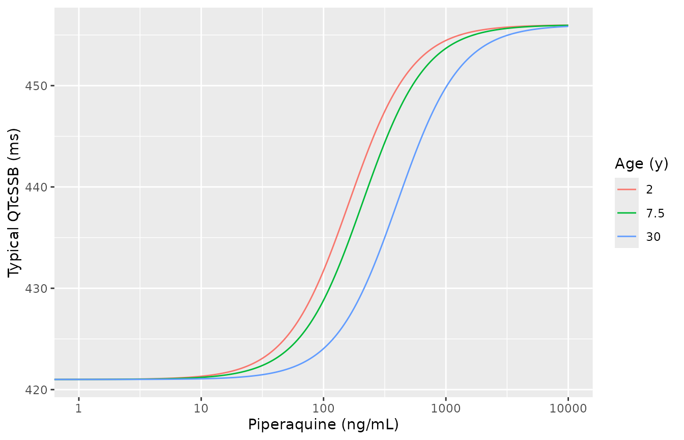
# Cross-check the closed form against the packaged model with IIV removed.
chk_ev <- data.frame(id = 1L, time = c(0, 0:24 * 4), evid = c(1L, rep(0L, 25)), amt = c(600, rep(0, 25)),
                     cmt = c("depot", rep("central", 25)), OCC = 1L, WT = 54, AGE = 7.5)
chk <- rxode2::rxSolve(rxode2::zeroRe(mod_qtc), events = chk_ev) |> as.data.frame()
#> Warning: some etas defaulted to non-mu referenced, possible parsing error: etaiov_fdepot_1, etaiov_fdepot_2, etaiov_fdepot_3, etaiov_mtt_1, etaiov_mtt_2, etaiov_mtt_3
#> as a work-around try putting the mu-referenced expression on a simple line
#> ℹ omega/sigma items treated as zero: 'etalfdepot', 'etalmtt', 'etalvc', 'etalvp', 'etalq2', 'etalvp2', 'etaiov_fdepot_1', 'etaiov_fdepot_2', 'etaiov_fdepot_3', 'etaiov_mtt_1', 'etaiov_mtt_2', 'etaiov_mtt_3', 'etae0', 'etalemax', 'etalec50'
closed <- 421 + 35 * chk$Cc^1.69 / (chk$Cc^1.69 + 209^1.69)
stopifnot(max(abs(chk$QTcS - closed)) < 1e-6)
Assumptions and deviations
- Form of the age effect on EC50. Tables 4 and S2 report ‘Effect of age on EC50 (%)’ as 4.10 and 2.87, but the equation is not printed in the paper or the supplement. The models use a linear effect centred on the study-median age of 7.5 years (Table 1): EC50_i = EC50 * (1 + theta * (AGE - 7.5)) * exp(eta). This form matches the Discussion statement that EC50 is lower in young children than in adults. It also reproduces the paper’s simulated median QTcmax (440-441 ms) and median DeltaQTcmax (16.8-18.5 ms) to within a few ms in the scenario table above. The centring value is the maintainers’ choice, and a different centre would rescale the typical EC50 at a given age.
- Residual error scale. The footnotes to Tables 4 and S2 describe sigma as an ‘additive residual error (variance)’, but the rows are labelled in ms. The models read 11.6 ms and 12.6 ms as standard deviations; as variances they would imply implausibly small residual SDs of 3.4 and 3.5 ms. The PK sigma (0.198) carries no unit and is a variance on the log scale, following the Table 2 footnote. The PK model’s propSd is therefore sqrt(0.198).
- Additive baseline IIV. The 17.0 ms and 10.6 ms baseline IIVs are standard deviations on the arithmetic scale (footnotes d and c). The Discussion’s ‘interindividual variability of +/- 17.0 ms’ supports this reading.
-
Dose-occasion effect on F. The fixed 0.237
increment is encoded additively, F = 1 + 0.237 * (OCC - 1), as in the
Hoglund 2017 prior model
(
modellib('Hoglund_2017_piperaquine')). For monthly courses,OCCrestarts at 1 at the start of each course. The paper does not state how its MDA simulation handled the occasion effect across courses. -
Between-occasion variability. IOV on F and MTT
(Equation 2) is implemented for three dose occasions, with one eta per
occasion multiplexed on
OCCand sharing a variance. - No IIV on CL/F or Q1/F. Table 2 reports none, and none is added.
- Dose basis. Doses in the model are piperaquine base, converted from piperaquine phosphate with the 57.7% factor of the Hoglund 2017 prior; this paper does not restate the conversion. The Figure 1 VPC comparison above supports base dosing. With phosphate doses, the simulated medians would be about 1.7-fold higher than the observed ones.
- Table 2 confidence intervals. For Vp2 IIV (31.8%, CI 32.0-33.3) and F IOV (42.8%, CI 43.5-47.8), the point estimate falls outside the printed bootstrap interval. The point estimates are used as printed.
- Age-weight relationship. Both virtual cohorts derive weight from age, or age from weight, using an approximate median weight-for-age curve chosen by the maintainers. The paper used the empirical relationship in its study population, which is not published.
- Sub-models not shipped. Table S1 gives linear DeltaQTc models for four heart-rate corrections (QTcF, QTcB, QTcSSB, QTcDAYS; for example, 5.90 ms per 100 ng/mL for QTcSSB, as quoted in the Abstract). These compared correction methods and were superseded by the Emax DeltaQTc model of Table S2, which is shipped. The linear absolute-QTc model (4.87 ms per 100 ng/mL) was likewise superseded by the Table 4 Emax model. The potassium effect on the QTc baseline was dropped from the final model by the authors and is not included.