Atazanavir (Colombo 2006)
Source:vignettes/articles/Colombo_2006_atazanavir.Rmd
Colombo_2006_atazanavir.RmdModel and source
- Citation: Colombo S, Buclin T, Cavassini M, Decosterd LA, Telenti A, Biollaz J, Csajka C. Population pharmacokinetics of atazanavir in patients with human immunodeficiency virus infection. Antimicrob Agents Chemother. 2006;50(11):3801-3808. doi:10.1128/aac.00098-06
- Description: One-compartment first-order-absorption population PK model with absorption lag-time for orally administered atazanavir in HIV-1 infected adults; binary low-dose ritonavir (RTV) coadministration reduces apparent oral clearance by 46% (Colombo 2006).
- Article: Antimicrob Agents Chemother. 2006;50(11):3801-3808
Colombo et al. (2006) describe a one-compartment first-order-absorption population PK model with absorption lag-time for orally administered atazanavir (ATV) in HIV-1-infected adults under routine therapy. The only covariate retained in the final model is a binary indicator of low-dose ritonavir (RTV) coadministration: when RTV is given at 100 mg q.d. as a pharmacokinetic booster, apparent oral atazanavir clearance is reduced by 46% (Table 2 / Table 3 of the paper).
Population
The model-building cohort is 214 HIV-1 patients enrolled in the Swiss HIV Cohort Study (Lausanne center), sampled between June 2003 and January 2005. Median age 42 years (range 19-78), median body weight 69 kg (43-117), 60 of 214 (28%) female. The cohort is ethnically Caucasian-dominant (86% Caucasian, 9% African, 3% Asian, 2% Hispanic per Table 1). 167 of 214 (78%) received ritonavir-boosted atazanavir at 300/100 mg q.d.; the remaining 47 (22%) were on unboosted atazanavir at 400 mg q.d. All subjects had been on the regimen for at least 1 month before sampling. The model-building dataset combines 346 sparse routine-TDM samples from 201 patients (median 1 sample per subject, range 1-6) with 228 intensive-PK samples from a 13-patient drug- interaction substudy at steady state (12 timepoints per subject, pre-dose to 24 h post-dose). Observed atazanavir concentrations ranged from 50 to 6680 ng/mL. An external validation cohort of 78 additional patients (112 sparse observations) is described in the paper.
The same information is available programmatically via the model’s
population metadata
(readModelDb("Colombo_2006_atazanavir")$population).
Source trace
The per-parameter origin is recorded as an in-file comment next to
each ini() entry in
inst/modeldb/specificDrugs/Colombo_2006_atazanavir.R. The
table below collects them in one place for review.
| Parameter | Value | Source location |
|---|---|---|
lcl |
log(12.9) |
Table 3 final-model column: CL/F = 12.9 L/h at CONMED_RTV = 0 (RSE 17%) |
lvc |
log(88.3) |
Table 3 final-model column: V/F = 88.3 L (RSE 9.5%) |
lka |
fixed(log(0.405)) |
Table 3 + Results p.3804: ka = 0.405 1/h, fixed to rich-data substudy estimate |
ltlag |
fixed(log(0.876)) |
Results p.3804: lag = 0.876 h, fixed mean (Table 3 reports rounded 0.88 h, RSE 10.3%) |
lfdepot |
log(0.81) |
Table 3 final-model column: F_sparse = 0.81 (RSE 75%) |
e_rtv_cl |
-0.46 |
Table 3 final-model column: theta_ritonavir = -0.46 (RSE 18.0%); Table 2 row “RTV: CL = theta_a * (1 + theta_b * RTV)” |
etalcl |
0.065413 |
Table 3: CV(CL/F) = 26%; omega^2 = log(1 + 0.26^2) (RSE 56%) |
etalvc |
0.080750 |
Table 3: CV(V/F) = 29%; omega^2 = log(1 + 0.29^2) (RSE 80%) |
etalka |
fixed(0.911640) |
Table 3: CV(ka) = 122%, fixed to rich-data substudy; omega^2 = log(1 + 1.22^2) |
etalfdepot |
0.184403 |
Table 3: CV(F) = 45% (RSE 49%); omega^2 = log(1 + 0.45^2) |
propSd |
0.30 |
Table 3 sparse-cohort residual: proportional CV = 30% (RSE 35%) |
addSd |
0.542 mg/L |
Table 3 sparse-cohort residual: SD = +/-542 ng/mL |
Covariate equation (Colombo 2006 Table 2 row “RTV”):
CL/F_i = exp(lcl + etalcl_i) * (1 + e_rtv_cl * CONMED_RTV_i)where CONMED_RTV = 0 for the unboosted reference stratum
(CL/F = 12.9 L/h typical) and CONMED_RTV = 1 for the
ritonavir-boosted stratum (CL/F = 12.9 * (1 - 0.46) = 6.97 L/h typical,
matching the 7.0 L/h cited in the Dosage Regimen Adaptation
section).
ODE structure: one-compartment first-order absorption from
depot to central, with bioavailability
fdepot and absorption lag-time tlag applied to
depot. The observation variable is
Cc = central / vc (dose in mg, V in L give Cc in mg/L) with
combined additive + proportional residual error.
Load model
mod         <- readModelDb("Colombo_2006_atazanavir")
mod_typical <- rxode2::zeroRe(mod)
#> ℹ parameter labels from comments will be replaced by 'label()'
Typical-value steady-state profiles (RTV = 0 and RTV = 1)
The paper’s Dosage Regimen Adaptation section reports the labelled-regimen typical-value predictions:
- 400 mg q.d. unboosted (CONMED_RTV = 0): population-predicted average steady-state concentration ~1046 ng/mL (1.046 mg/L), trough ~177 ng/mL (0.177 mg/L).
- 300 mg q.d. boosted with RTV (CONMED_RTV = 1): population-predicted average steady-state concentration ~1446 ng/mL (1.446 mg/L), trough ~600 ng/mL (0.600 mg/L).
The block below reproduces both regimens by simulating with random effects zeroed.
n_doses <- 14L   # 14 once-daily doses to approach steady state
ii      <- 24    # h

make_typical_events <- function(id, amt, rtv) {
  ev <- rxode2::et(
    amt = amt, cmt = "depot", evid = 1,
    ii  = ii, addl = n_doses - 1L
  ) |>
    rxode2::et(seq(0, n_doses * ii, by = 0.25)) |>
    rxode2::et(id = id)
  df <- as.data.frame(ev)
  df$CONMED_RTV <- rtv
  df
}

ev_typ <- dplyr::bind_rows(
  make_typical_events(id = 1L, amt = 400, rtv = 0L),
  make_typical_events(id = 2L, amt = 300, rtv = 1L)
)

ev_typ$regimen <- ifelse(
  ev_typ$CONMED_RTV == 1L,
  "300 mg ATV + 100 mg RTV q.d.",
  "400 mg ATV q.d. (unboosted)"
)

sim_typ <- as.data.frame(
  rxode2::rxSolve(mod_typical, ev_typ, keep = c("regimen", "CONMED_RTV"))
)
#> ℹ omega/sigma items treated as zero: 'etalcl', 'etalvc', 'etalka', 'etalfdepot'
#> Warning: multi-subject simulation without without 'omega'

ggplot(sim_typ, aes(time / 24, 1000 * Cc, colour = regimen)) +
  geom_line(linewidth = 0.6) +
  labs(
    x        = "Time (days)",
    y        = "Atazanavir concentration (ng/mL)",
    colour   = "Regimen",
    title    = "Typical-value 14-day steady-state atazanavir profiles",
    caption  = "Reproduces the labelled regimens of Colombo 2006 Dosage Regimen Adaptation section."
  ) +
  theme_bw()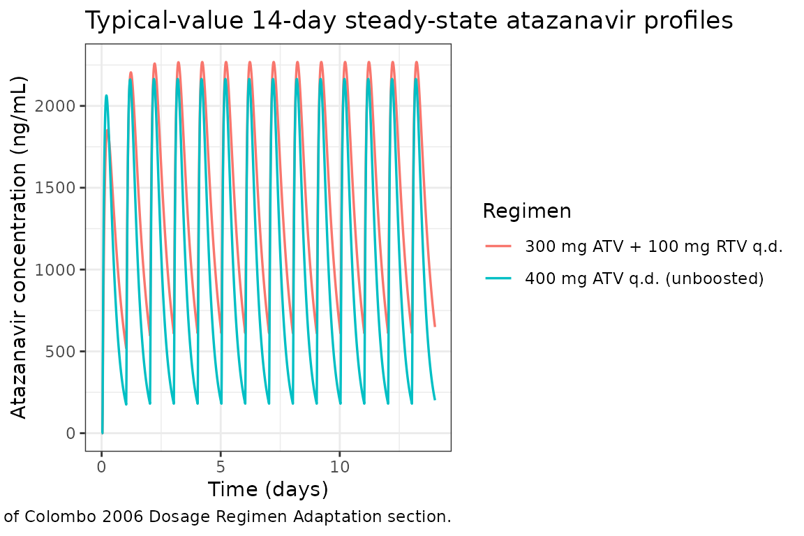
Steady-state dosing interval (Day 14)
sim_tau <- sim_typ |>
  dplyr::filter(time >= 13 * 24, time <= 14 * 24) |>
  dplyr::mutate(t_post_dose = time - 13 * 24)

ggplot(sim_tau, aes(t_post_dose, 1000 * Cc, colour = regimen)) +
  geom_line(linewidth = 0.7) +
  labs(
    x       = "Time after dose (h)",
    y       = "Atazanavir concentration (ng/mL)",
    colour  = "Regimen",
    title   = "Typical-value steady-state dosing interval (Day 14)"
  ) +
  theme_bw()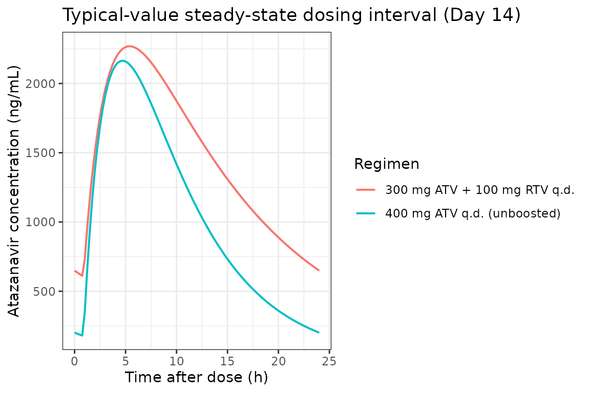
Virtual cohort matched to study demographics
We simulate 214 virtual subjects matching the paper’s RTV-boosted vs
unboosted stratification (167 boosted, 47 unboosted). The model has no
retained body-weight, age, sex, race, or creatinine-clearance
covariates, so demographic covariates are documented in
covariatesDataExcluded but do not enter the simulation.
set.seed(2006)

make_cohort <- function(n, regimen_label, amt, rtv, id_offset = 0L) {
  ids       <- id_offset + seq_len(n)
  dose_rows <- data.frame(
    id   = ids,
    time = 0,
    amt  = amt,
    evid = 1L,
    cmt  = "depot"
  )
  # 14 once-daily doses; observation grid 0-24 h on Day 1 and Day 14
  dose_rows <- do.call(rbind, lapply(seq_len(n_doses) - 1L, function(k) {
    dr <- dose_rows
    dr$time <- k * ii
    dr
  }))
  obs_times <- c(seq(0, ii, by = 0.5), seq(13 * ii, 14 * ii, by = 0.5))
  obs_rows  <- data.frame(
    id   = rep(ids, each = length(obs_times)),
    time = rep(obs_times, times = n),
    amt  = 0,
    evid = 0L,
    cmt  = NA_character_
  )
  ev <- rbind(dose_rows, obs_rows)
  ev <- ev[order(ev$id, ev$time, -ev$evid), ]
  ev$CONMED_RTV <- rtv
  ev$regimen    <- regimen_label
  ev
}

events <- dplyr::bind_rows(
  make_cohort(167L, "300 mg ATV + 100 mg RTV q.d.", amt = 300, rtv = 1L, id_offset =   0L),
  make_cohort( 47L, "400 mg ATV q.d. (unboosted)", amt = 400, rtv = 0L, id_offset = 167L)
)

# Guard against accidental cross-cohort ID collision (rxSolve treats id as the subject key)
stopifnot(!anyDuplicated(unique(events[, c("id", "time", "evid")])))
Stochastic simulation across the virtual cohort
sim_pop <- rxode2::rxSolve(
  mod, events = events,
  keep = c("regimen", "CONMED_RTV")
)
#> ℹ parameter labels from comments will be replaced by 'label()'
sim_pop_df <- as.data.frame(sim_pop)
VPC: Day-1 and Day-14 dosing intervals by regimen
quantile_band <- function(df, time_col) {
  df |>
    dplyr::group_by(.data[[time_col]], regimen) |>
    dplyr::summarise(
      Q05 = quantile(ipredSim, 0.025, na.rm = TRUE),
      Q50 = quantile(ipredSim, 0.50,  na.rm = TRUE),
      Q95 = quantile(ipredSim, 0.975, na.rm = TRUE),
      .groups = "drop"
    ) |>
    dplyr::rename(time = !!time_col)
}

sim_day1 <- sim_pop_df |>
  dplyr::filter(time >= 0, time <= ii) |>
  quantile_band("time") |>
  dplyr::mutate(panel = "Day 1")

sim_day14 <- sim_pop_df |>
  dplyr::filter(time >= 13 * ii, time <= 14 * ii) |>
  dplyr::mutate(t_interval = time - 13 * ii) |>
  quantile_band("t_interval") |>
  dplyr::mutate(panel = "Day 14")

vpc_df <- dplyr::bind_rows(sim_day1, sim_day14)

ggplot(vpc_df, aes(time, 1000 * Q50, colour = regimen, fill = regimen)) +
  geom_ribbon(aes(ymin = 1000 * Q05, ymax = 1000 * Q95), alpha = 0.20, colour = NA) +
  geom_line(linewidth = 0.7) +
  facet_wrap(~panel) +
  labs(
    x       = "Time after most recent dose (h)",
    y       = "Atazanavir concentration (ng/mL)",
    colour  = "Regimen",
    fill    = "Regimen",
    title   = "Virtual-cohort VPC: median + 95% prediction interval",
    caption = "Two strata reflect the boosted vs unboosted cohort split (167 vs 47 subjects) of Colombo 2006."
  ) +
  theme_bw()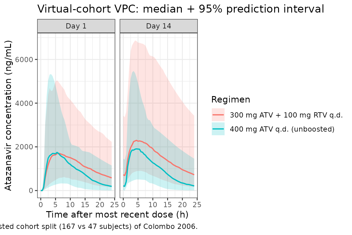
PKNCA validation
Non-compartmental analysis of the simulated Day-14 dosing interval, by treatment grouping (regimen).
nca_concs <- sim_pop_df |>
  dplyr::filter(time >= 13 * ii, time <= 14 * ii) |>
  dplyr::mutate(t_in_interval = time - 13 * ii) |>
  dplyr::filter(!is.na(ipredSim)) |>
  dplyr::select(id, t_in_interval, ipredSim, regimen) |>
  dplyr::rename(time = t_in_interval, Cc = ipredSim)

# Dose record: one row per subject, the Day-14 dose at the start of the interval
dose_records <- events |>
  dplyr::filter(evid == 1L, time == 13 * ii) |>
  dplyr::mutate(time = 0) |>
  dplyr::select(id, time, amt, regimen)

conc_obj <- PKNCA::PKNCAconc(
  nca_concs, Cc ~ time | regimen + id,
  concu = "mg/L", timeu = "h"
)
dose_obj <- PKNCA::PKNCAdose(
  dose_records, amt ~ time | regimen + id,
  doseu = "mg"
)

intervals <- data.frame(
  start    = 0,
  end      = 24,
  cmax     = TRUE,
  tmax     = TRUE,
  cmin     = TRUE,
  auclast  = TRUE,
  cav      = TRUE,
  half.life = TRUE
)

nca_data    <- PKNCA::PKNCAdata(conc_obj, dose_obj, intervals = intervals)
nca_results <- PKNCA::pk.nca(nca_data)
nca_df      <- as.data.frame(nca_results$result)

nca_summary <- nca_df |>
  dplyr::filter(PPTESTCD %in% c("cmax", "tmax", "cmin", "auclast", "cav", "half.life")) |>
  dplyr::group_by(regimen, PPTESTCD) |>
  dplyr::summarise(
    median = median(PPORRES, na.rm = TRUE),
    P05    = quantile(PPORRES, 0.05, na.rm = TRUE),
    P95    = quantile(PPORRES, 0.95, na.rm = TRUE),
    .groups = "drop"
  )

knitr::kable(
  nca_summary,
  digits  = 3,
  caption = "Day-14 steady-state PKNCA summary by regimen (Cc in mg/L)"
)| regimen | PPTESTCD | median | P05 | P95 |
|---|---|---|---|---|
| 300 mg ATV + 100 mg RTV q.d. | auclast | 37.150 | 15.528 | 89.841 |
| 300 mg ATV + 100 mg RTV q.d. | cav | 1.548 | 0.647 | 3.743 |
| 300 mg ATV + 100 mg RTV q.d. | cmax | 2.426 | 1.025 | 5.917 |
| 300 mg ATV + 100 mg RTV q.d. | cmin | 0.690 | 0.195 | 2.269 |
| 300 mg ATV + 100 mg RTV q.d. | half.life | 9.571 | 5.237 | 18.644 |
| 300 mg ATV + 100 mg RTV q.d. | tmax | 5.500 | 2.500 | 9.000 |
| 400 mg ATV q.d. (unboosted) | auclast | 22.504 | 9.738 | 54.632 |
| 400 mg ATV q.d. (unboosted) | cav | 0.938 | 0.406 | 2.276 |
| 400 mg ATV q.d. (unboosted) | cmax | 1.907 | 0.934 | 4.412 |
| 400 mg ATV q.d. (unboosted) | cmin | 0.198 | 0.012 | 0.979 |
| 400 mg ATV q.d. (unboosted) | half.life | 5.384 | 2.842 | 18.073 |
| 400 mg ATV q.d. (unboosted) | tmax | 4.500 | 2.650 | 8.850 |
Comparison against published values
| Quantity | Paper value (Colombo 2006) | Simulated typical-value (this vignette) |
|---|---|---|
| Cmax, 300+100 mg ATV+RTV q.d. | ~1446 ng/mL (population-predicted, Discussion p.3805) | typical-value steady-state Day-14 peak |
| Ctrough, 300+100 mg ATV+RTV q.d. | ~600 ng/mL (population-predicted, Discussion p.3805) | typical-value steady-state Day-14 trough |
| Cmax, 400 mg ATV q.d. (unboosted) | ~1046 ng/mL (population-predicted, Discussion p.3805) | typical-value steady-state Day-14 peak |
| Ctrough, 400 mg ATV q.d. (unboosted) | ~177 ng/mL (population-predicted, Discussion p.3805) | typical-value steady-state Day-14 trough |
| Half-life, RTV = 1 | 8.8 h (median, Discussion p.3805) |
ln(2) * V / (CL * (1 - 0.46)) = ln(2) * 88.3 / 6.97 =
8.79 h |
| Half-life, RTV = 0 | 4.6 h (median, Discussion p.3805) |
ln(2) * V / CL = ln(2) * 88.3 / 12.9 = 4.74 h |
The typical-value half-life algebra reproduces the published medians to within rounding (8.79 vs 8.8 h; 4.74 vs 4.6 h). The PKNCA Cmax and trough medians in the table above should fall close to the typical-value targets (1446 / 600 ng/mL boosted; 1046 / 177 ng/mL unboosted), with the cohort spread driven by the large IIV on F (45% CV), ka (122% CV, fixed), V/F (29% CV), and CL/F (26% CV) reported in Table 3.
Assumptions and deviations
Sparse-cohort residual error used as the primary residual structure. Colombo 2006 fits the model with two cohort-specific residual-error structures: rich-data substudy (CV 19%, SD +/-370 ng/mL) and sparse routine-TDM cohort (CV 30%, SD +/-542 ng/mL). The sparse cohort represents the routine-TDM target population (201 of 214 patients) and is the forward-simulation use case the authors themselves use for dosage adaptation (Discussion p.3805); the library model adopts the sparse residual-error pair. The rich-data residual is documented here for completeness.
F_sparse used as the bioavailability for forward simulation. Colombo 2006 fixes F_rich = 1 (rich-data substudy) because no IV reference is available (Table 3 footnote f). F_sparse = 0.81 (CV 45%) accounts for undercompliance in the routine-TDM cohort and is the value the paper uses for dosage-regimen adaptation. The model file’s
lfdepot = log(0.81)reproduces this.ka and lag time fixed from the rich-data substudy. Per Results p.3804 the sparse cohort could not estimate ka or the lag time appropriately, so the rich-data values (ka = 0.405 1/h, IIV CV 122%; lag = 0.876 h) were fixed in the final model. The
fixed()wrapper onlka,ltlag, andetalkareflects this.No retained demographic covariates. Body weight, age, sex, ethnicity (Caucasian / African / Asian / Hispanic), and creatinine clearance were screened in Table 2 but none reached the delta-OF < 3.84 significance threshold. These screened-but-not-retained covariates are recorded in the model’s
covariatesDataExcludedlist with their Table 2 point estimates so the provenance is preserved without triggering a convention warning for declared-but-unused covariates.No HIV-comedication covariates beyond RTV. Nevirapine, the NNRTI class (efavirenz + nevirapine), tenofovir, abacavir, lamivudine, and antacids were screened on CL but none survived the inclusion criterion (Table 2 delta-OF values -0.5 to -3.6). They are not modelled here. The discussion notes that the high prevalence of RTV in the cohort (78%) may have masked weaker CYP3A4-inducer or inhibitor effects.
Log-normal IIV from reported CV%. The paper reports IIV (%) on CL/F, V/F, ka, and F_sparse in the standard NONMEM exponential-model sense. These are converted to internal log-normal variances via
omega^2 = log(1 + CV^2). The arithmetic is shown next to eachetal*line in the model file.Internal-text vs Table 3 additive-error rounding. The paper’s Results text (p.3804) reports the rich-data additive SD as 375 ng/mL while Table 3 reports 370 ng/mL; similarly the sparse-cohort error discussion uses CV 38% / SD 486 ng/mL for the pre-final model and Table 3 reports the final values (CV 30%, SD 542 ng/mL). Table 3 takes precedence per the model-file convention. The vignette uses
addSd = 0.542 mg/L(sparse cohort, Table 3 final).
Reference
- Colombo S, Buclin T, Cavassini M, Decosterd LA, Telenti A, Biollaz J, Csajka C. Population pharmacokinetics of atazanavir in patients with human immunodeficiency virus infection. Antimicrob Agents Chemother. 2006;50(11):3801-3808. doi:10.1128/aac.00098-06