Imeglimin (Tomita 2022)
Source:vignettes/articles/Tomita_2022_imeglimin.Rmd
Tomita_2022_imeglimin.RmdModel and source
mod <- readModelDb("Tomita_2022_imeglimin")
ui <- rxode2::rxode(mod)
#> ℹ parameter labels from comments will be replaced by 'label()'- Citation: Tomita Y, Hansson E, Mazuir F, Wellhagen GJ, Ooi QX, Mezzalana E, Kitamura A, Nemoto D, Bolze S. Imeglimin population pharmacokinetics and dose adjustment predictions for renal impairment in Japanese and Western patients with type 2 diabetes. Clin Transl Sci. 2022;15(4):1014-1026. doi:10.1111/cts.13221
- Description: Two-compartment population PK model for oral imeglimin in Japanese and Western healthy volunteers and patients with type 2 diabetes, including patients with chronic kidney disease down to eGFR 14 mL/min/1.73 m^2 (Tomita 2022). First-order absorption with a lag time; dose-dependent relative bioavailability (inhibitory Emax on dose, normalised to F = 1 at 1000 mg) and dose-dependent ka (power on dose); formulation and fasting effects on lag time and ka; linear eGFR effect on CL/F capped at 120 mL/min/1.73 m^2 plus power effects of body weight and age on CL/F, body weight on Vc/F, and age and Japanese ethnicity on Q/F. Log-scale residual error with separate magnitudes for phase I studies and for pre-dose samples. Doses must be supplied as imeglimin FREE BASE (labelled imeglimin hydrochloride mass x 0.810, e.g. 1000 mg tablet = 810 mg); the dose nonlinearity on F and ka is evaluated on the labelled dose, recovered in model() as podo(depot) / 0.810.
- Article: https://doi.org/10.1111/cts.13221 (open access, PMC9010270)
Population
Tomita et al. pooled 8256 imeglimin plasma concentrations from 867 individuals in nine clinical studies (Table 1): a single/multiple ascending dose study in Japanese and Western healthy volunteers, Western and Japanese renal-impairment studies, a study of Western patients with type 2 diabetes (T2DM) and CKD stages G3b-G4, two Western phase IIa studies, the Western and Japanese phase IIb studies, and the Japanese phase III monotherapy study TIMES 1. Two further Japanese phase III studies (TIMES 2, TIMES 3; 796 patients) were held out for external evaluation only. 745 of the 867 individuals had T2DM. Table 2 gives median (range) age 57 (20-75), 59 (20-75) and 63 (34-80) years, body weight 73.0 (42.4-148), 80.9 (35.6-135) and 69.1 (42.5-124) kg, and eGFR 77.6 (14.1-152), 83.8 (42.6-138) and 72.8 (47.2-106) mL/min/1.73 m^2 for the phase I (n = 160), phase II (n = 604) and TIMES 1 (n = 103) subsets. 43% were female and 44% were Japanese; the Western subjects were mostly White. Doses were 500-8000 mg single doses and 500-2000 mg b.i.d. or 1000-2000 mg q.d. of imeglimin hydrochloride, given as capsules, conventional tablets or the optimised tablet used in the Japanese phase IIb / III studies.
The same information is available programmatically via
ui$population.
Source trace
| Equation / parameter | Value | Source location |
|---|---|---|
| Two-compartment model, first-order absorption with lag | n/a | Results, ‘Population pharmacokinetic analysis’ |
lka |
log(0.144) 1/h | Table 3 |
ltlag |
log(0.229) h | Table 3 |
lfdepot |
fixed(log(1)) | Table 3 (F = 1 FIX) |
lcl |
log(66.9) L/h | Table 3 |
lvc |
log(142) L | Table 3 |
lq |
log(15.9) L/h | Table 3 |
lvp |
log(374) L | Table 3 |
ld50_fdepot, F(dose) |
log(2410) mg | Table 3; Equation 7, F = 1 - (Dose/(Dose + D50) - 1000/(1000 + D50)) |
e_dose_ka |
-0.138 | Table 3; Equation 1 with reference 1000 mg (Figure 1 caption) |
e_crcl_cl, eGFR on CL/F |
0.00951 | Table 3; Equation 8 (linear, centred at 81.4, capped at 120) |
e_wt_cl |
0.388 | Table 3; Equation 9, reference 77.35 kg (Table 3 footnote) |
e_age_cl |
-0.343 | Table 3; Equation 10, reference 59 years (Table 3 footnote) |
e_wt_vc |
0.802 | Table 3; Equation 1 |
e_age_q |
-0.859 | Table 3; Equation 1 |
e_japanese_q |
-0.291 | Table 3; Equation 2 |
e_capsule_tlag |
2.45 | Table 3 (footnote a: relative to the optimised tablet); Equation 2 |
e_convtab_tlag |
0.719 | Table 3; Equation 2 |
e_capsconv_ka |
0.298 | Table 3; Equation 2 |
e_fasted_tlag |
-0.449 | Table 3 (footnote b: relative to non-fasting); Equation 2 |
e_fasted_ka |
0.389 | Table 3; Equation 2 |
etalka |
0.228^2 | Table 3 ‘IIV of ka (CV)’ |
etalcl, etalfdepot block |
0.461^2, 0.821 x 0.461 x 0.529, 0.529^2 | Table 3 ‘IIV of CL’, ‘IIV of F’, ‘Correlation CL/F’ |
etalvc |
0.645^2 | Table 3 |
etalvp |
0.605^2 | Table 3 |
expSdPhase23 |
0.359 | Table 3 ‘Proportional RUV (CV)’; Methods (additive on log scale) |
expSdPhase1 |
0.190 | Table 3 ‘Proportional phase I RUV (CV)’ |
expSdPredose |
0.505 | Table 3 ‘Proportional predose RUV (CV)’ |
| Salt factor 0.810 | n/a | Methods ‘Clinical studies’; Equation 4 |
Dose nonlinearity on F (Equation 7)
The Figure 3 caption converts the mass-balance bioavailability at
1000 mg (0.439) to 0.492 at 500 mg “using the inhibitory maximum effect
function for F in population pharmacokinetic (PK) model (Equation 7)”.
That is a printed answer key for Equation 7 and for the labelled-dose
reading of Dose.
covs_ref <- data.frame(
  CRCL = 81.4, WT = 77.35, AGE = 59, RACE_JAPANESE = 0, FORM_CAPSULE = 0,
  FORM_IMEGLIMIN_CONVENTIONAL_TABLET = 0, FED = 1, STUDY_IMEGLIMIN_PHASE1 = 0,
  SAMPLE_PREDOSE = 0
)
mod_typ <- rxode2::zeroRe(mod)
#> ℹ parameter labels from comments will be replaced by 'label()'
#> Warning: No sigma parameters in the model

# One dose per subject; the labelled dose is amt / 0.810 (amt = free base).
labelled <- c(250, 500, 1000, 1500, 2000, 4000, 8000)
ev_f <- data.frame(
  id = rep(seq_along(labelled), each = 2),
  time = rep(c(0, 1), length(labelled)),
  evid = rep(c(1L, 0L), length(labelled)),
  amt = rep(c(1, 0), length(labelled)) * rep(labelled * 0.810, each = 2),
  cmt = "depot"
) |>
  cbind(covs_ref)
f_sim <- rxode2::rxSolve(mod_typ, ev_f, returnType = "data.frame") |>
  dplyr::distinct(id, fdepot, ka) |>
  dplyr::mutate(labelled_dose = labelled[id])
#> ℹ omega/sigma items treated as zero: 'etalka', 'etalcl', 'etalfdepot', 'etalvc', 'etalvp'
#> Warning: multi-subject simulation without without 'omega'

f500 <- f_sim$fdepot[f_sim$labelled_dose == 500]
f1000 <- f_sim$fdepot[f_sim$labelled_dose == 1000]
c(F_500 = f500, F_1000 = f1000, ratio_model = f500 / f1000, ratio_paper = 0.492 / 0.439)
#>       F_500      F_1000 ratio_model ratio_paper
#>    1.121434    1.000000    1.121434    1.120729
# Deterministic: the model ratio is 1.1214; the paper's two printed values
# (3 significant figures) give 1.1207.
stopifnot(abs(f1000 - 1) < 1e-10, abs(f500 / f1000 / (0.492 / 0.439) - 1) < 0.002)
ggplot(f_sim, aes(labelled_dose, fdepot)) +
  geom_line() +
  geom_point() +
  geom_vline(xintercept = 1000, colour = "red") +
  labs(x = "Imeglimin hydrochloride dose (mg)", y = "Relative bioavailability F")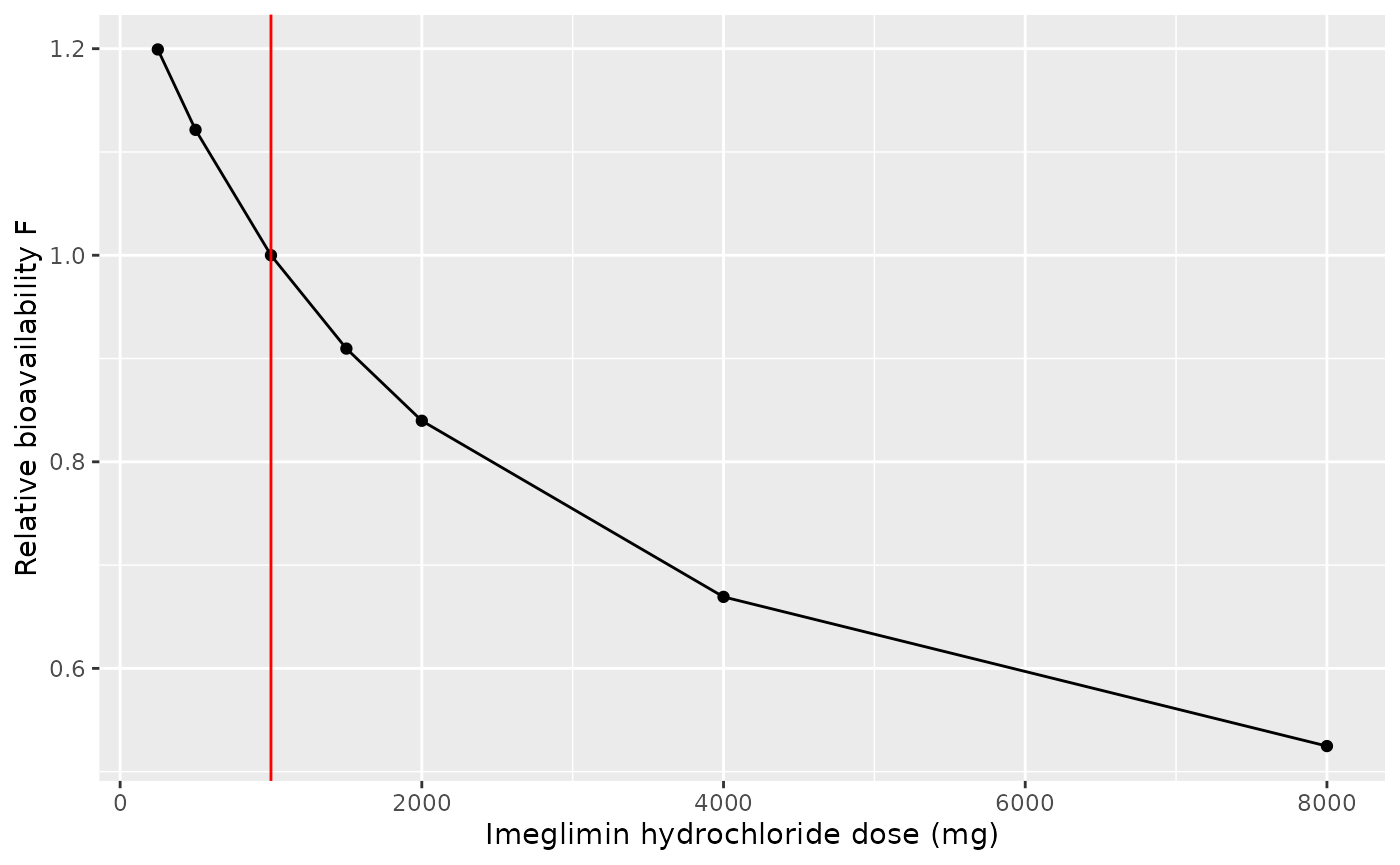
Replicates Figure 1d of Tomita 2022: relative bioavailability versus labelled dose (other covariates at the reference).
Covariate effects on CL/F (Figure 1a-c)
grid_cov <- dplyr::bind_rows(
  data.frame(panel = "eGFR (mL/min/1.73 m^2)", x = seq(14, 152, by = 2)) |>
    dplyr::mutate(CRCL = x, WT = 77.35, AGE = 59),
  data.frame(panel = "Body weight (kg)", x = seq(35, 148, by = 2)) |>
    dplyr::mutate(CRCL = 81.4, WT = x, AGE = 59),
  data.frame(panel = "Age (years)", x = seq(20, 80, by = 1)) |>
    dplyr::mutate(CRCL = 81.4, WT = 77.35, AGE = x)
) |>
  dplyr::mutate(id = dplyr::row_number())
ev_cov <- grid_cov |>
  dplyr::select(id, CRCL, WT, AGE) |>
  dplyr::mutate(
    time = 1, evid = 0L, amt = 0, cmt = "central", RACE_JAPANESE = 0, FORM_CAPSULE = 0,
    FORM_IMEGLIMIN_CONVENTIONAL_TABLET = 0, FED = 1, STUDY_IMEGLIMIN_PHASE1 = 0,
    SAMPLE_PREDOSE = 0
  )
cl_sim <- rxode2::rxSolve(mod_typ, ev_cov, returnType = "data.frame") |>
  dplyr::select(id, cl) |>
  dplyr::left_join(grid_cov, by = "id")
#> ℹ omega/sigma items treated as zero: 'etalka', 'etalcl', 'etalfdepot', 'etalvc', 'etalvp'
#> Warning: multi-subject simulation without without 'omega'

# Closed form of Equations 8-10 from the printed constants.
cl_closed <- 66.9 * (1 + (pmin(cl_sim$CRCL, 120) - 81.4) * 0.00951) *
  (cl_sim$WT / 77.35)^0.388 * (cl_sim$AGE / 59)^-0.343
stopifnot(max(abs(cl_sim$cl / cl_closed - 1)) < 1e-10)
# The eGFR cap: CL/F is flat above 120 mL/min/1.73 m^2.
stopifnot(abs(cl_sim$cl[cl_sim$panel == "eGFR (mL/min/1.73 m^2)" & cl_sim$x == 150] /
  cl_sim$cl[cl_sim$panel == "eGFR (mL/min/1.73 m^2)" & cl_sim$x == 120] - 1) < 1e-10)

ggplot(cl_sim, aes(x, cl)) +
  geom_line() +
  facet_wrap(~panel, scales = "free_x") +
  labs(x = NULL, y = "Typical CL/F (L/h)")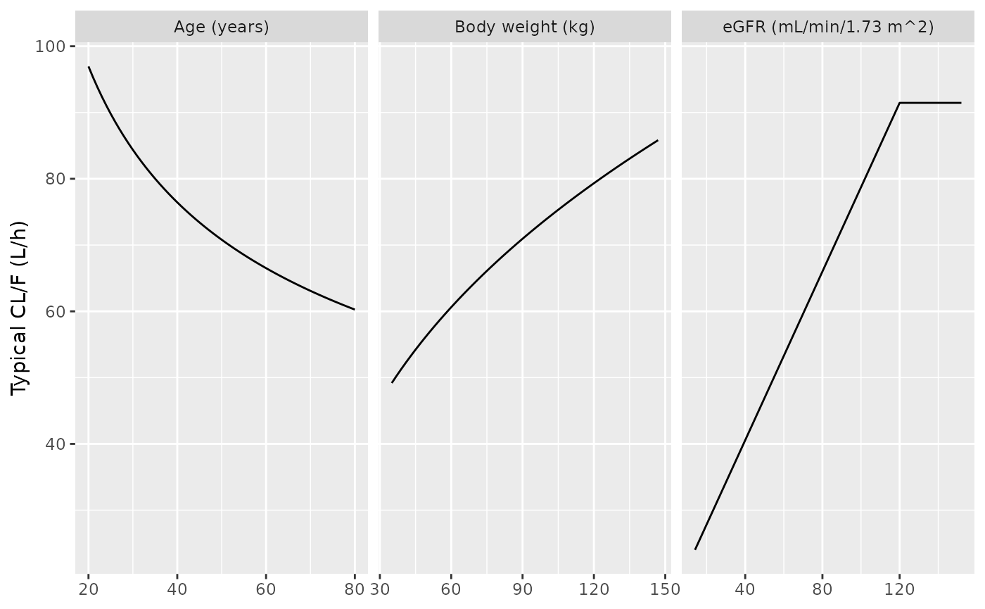
Replicates Figure 1a-c of Tomita 2022: CL/F against eGFR, body weight and age, one covariate varied at a time (others at the reference: 77.35 kg, 81.4 mL/min/1.73 m^2, 59 years).
Virtual cohorts for Table 4
Table 4 of the paper reports the steady-state AUC over 24 h (free base, ug h/mL) for virtual Japanese reference patients resampled from the Japanese phase IIb and TIMES 1 studies, for the same patients with eGFR replaced by a uniform draw over CKD stages G3a (45-60), G3b (30-45) and G4 (15-30) and age increased by 5.5 or 7.8 years, and for Western patients from the Western phase IIb study, alone or with eGFR lowered by 15.24 mL/min/1.73 m^2 and body weight by 17.5 kg. The individual covariate data are not public, so the cohorts below are drawn from truncated distributions matching the medians and ranges printed in Table 4. All simulations use the optimised tablet under non-fasting conditions, as the paper’s simulations did. Each arm has 200 subjects.
# Draw n values from a distribution and redraw any value outside [lo, hi].
rtrunc <- function(n, draw, lo, hi) {
  x <- draw(n)
  bad <- x < lo | x > hi
  while (any(bad)) {
    x[bad] <- draw(sum(bad))
    bad <- x < lo | x > hi
  }
  x
}

draw_age_jp <- function(n) rnorm(n, 62, 10)
draw_wt_jp <- function(n) rlnorm(n, log(68.8), 0.18)
draw_egfr_jp <- function(n) rlnorm(n, log(72.6), 0.2)
draw_age_w <- function(n) rnorm(n, 59, 10)
draw_wt_w <- function(n) rlnorm(n, log(85.8), 0.2)
draw_egfr_w <- function(n) rlnorm(n, log(92.8), 0.17)

# Build the dosing + observation records of one arm: b.i.d. dosing of the
# labelled dose for 14 days (28 doses), observations over the last 24 h.
make_arm <- function(covs, labelled_dose, arm, id_offset) {
  n <- nrow(covs)
  covs <- covs |>
    dplyr::mutate(
      id = id_offset + seq_len(n), arm = arm, labelled_dose = labelled_dose,
      FORM_CAPSULE = 0, FORM_IMEGLIMIN_CONVENTIONAL_TABLET = 0, FED = 1,
      STUDY_IMEGLIMIN_PHASE1 = 0, SAMPLE_PREDOSE = 0
    )
  dose_times <- seq(0, 324, by = 12)
  obs_times <- 312 + c(0, 0.5, 1, 1.5, 2, 2.5, 3, 4, 5, 6, 8, 10, 12)
  obs_times <- sort(unique(c(obs_times, obs_times + 12)))
  doses <- tidyr::expand_grid(id = covs$id, time = dose_times) |>
    dplyr::mutate(evid = 1L, amt = labelled_dose * 0.810, cmt = "depot")
  obs <- tidyr::expand_grid(id = covs$id, time = obs_times) |>
    dplyr::mutate(evid = 0L, amt = 0, cmt = "central")
  dplyr::bind_rows(doses, obs) |>
    dplyr::left_join(covs, by = "id") |>
    dplyr::arrange(id, time, dplyr::desc(evid))
}
set.seed(20220401)
n_arm <- 200
jp_ref <- data.frame(
  AGE = rtrunc(n_arm, draw_age_jp, 32, 83),
  WT = rtrunc(n_arm, draw_wt_jp, 35.6, 124),
  CRCL = rtrunc(n_arm, draw_egfr_jp, 47.2, 138),
  RACE_JAPANESE = 1
)
jp_g3a <- jp_ref |> dplyr::mutate(CRCL = runif(n_arm, 45, 60), AGE = AGE + 5.5)
jp_g3b <- jp_ref |> dplyr::mutate(CRCL = runif(n_arm, 30, 45), AGE = AGE + 7.8)
jp_g4 <- jp_ref |> dplyr::mutate(CRCL = runif(n_arm, 15, 30), AGE = AGE + 7.8)
w_ref <- data.frame(
  AGE = rtrunc(n_arm, draw_age_w, 20, 75),
  WT = rtrunc(n_arm, draw_wt_w, 54, 135),
  CRCL = rtrunc(n_arm, draw_egfr_w, 47.3, 125),
  RACE_JAPANESE = 0
)
w_egfr <- w_ref |> dplyr::mutate(CRCL = CRCL - 15.24)
w_egfr_wt <- w_egfr |> dplyr::mutate(WT = WT - 17.5)

arm_def <- tibble::tribble(
  ~arm,                                   ~cohort,      ~dose,
  "Japanese reference, 1000 mg b.i.d.",    "jp_ref",     1000,
  "Japanese reference, 500 mg b.i.d.",     "jp_ref",     500,
  "CKD G3a, 1000 mg b.i.d.",               "jp_g3a",     1000,
  "CKD G3a, 500 mg b.i.d.",                "jp_g3a",     500,
  "CKD G3b, 1000 mg b.i.d.",               "jp_g3b",     1000,
  "CKD G3b, 500 mg b.i.d.",                "jp_g3b",     500,
  "CKD G4, 1000 mg b.i.d.",                "jp_g4",      1000,
  "CKD G4, 500 mg b.i.d.",                 "jp_g4",      500,
  "Western reference, 2000 mg b.i.d.",     "w_ref",      2000,
  "Western reference, 1500 mg b.i.d.",     "w_ref",      1500,
  "Western reference, 1000 mg b.i.d.",     "w_ref",      1000,
  "Western similar eGFR, 1500 mg b.i.d.",  "w_egfr",     1500,
  "Western similar eGFR and weight, 1500 mg b.i.d.", "w_egfr_wt", 1500
)
cohorts <- list(
  jp_ref = jp_ref, jp_g3a = jp_g3a, jp_g3b = jp_g3b, jp_g4 = jp_g4,
  w_ref = w_ref, w_egfr = w_egfr, w_egfr_wt = w_egfr_wt
)
events <- dplyr::bind_rows(lapply(seq_len(nrow(arm_def)), function(i) {
  make_arm(cohorts[[arm_def$cohort[i]]], arm_def$dose[i], arm_def$arm[i], (i - 1L) * n_arm)
}))
stopifnot(!anyDuplicated(unique(events[, c("id", "time", "evid")])))
Simulation
rxode2::rxSetSeed(20220401)
sim <- rxode2::rxSolve(
  mod, events = events, keep = c("arm", "labelled_dose"),
  returnType = "data.frame", maxsteps = 1e6
)
#> ℹ parameter labels from comments will be replaced by 'label()'
stopifnot(!anyNA(sim$Cc))
sim |>
  dplyr::filter(grepl("1000 mg", arm), !grepl("Western", arm)) |>
  dplyr::group_by(arm, time) |>
  dplyr::summarise(
    Q05 = quantile(Cc, 0.05), Q50 = median(Cc), Q95 = quantile(Cc, 0.95),
    .groups = "drop"
  ) |>
  ggplot(aes(time - 312, Q50, colour = arm, fill = arm)) +
  geom_ribbon(aes(ymin = Q05, ymax = Q95), alpha = 0.15, colour = NA) +
  geom_line() +
  scale_y_log10() +
  labs(x = "Time after the dose at day 14 (h)", y = "Imeglimin (ug/mL, free base)", colour = NULL, fill = NULL)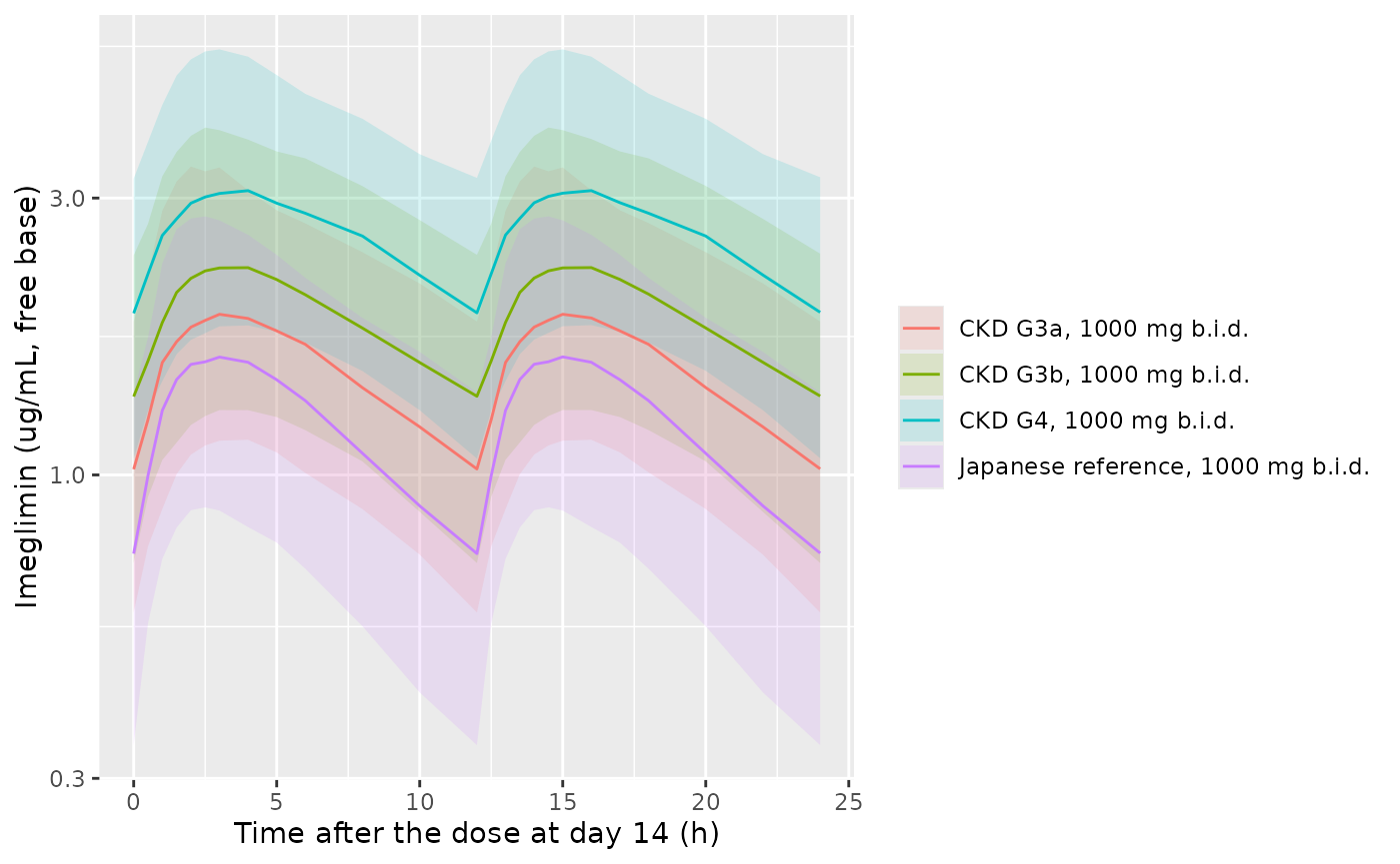
Simulated steady-state imeglimin concentrations (median and 5th-95th percentiles) over the last 24 h of 1000 mg b.i.d. in Japanese patients by CKD stage.
PKNCA validation
AUC over the last 24 h of b.i.d. dosing (two dosing intervals) is the paper’s AUC24,ss. PKNCA is run once per arm (one call with all 2600 subjects is slow).
sim_nca <- sim |>
  dplyr::filter(!is.na(Cc)) |>
  dplyr::select(id, time, Cc, arm)
dose_df <- events |>
  dplyr::filter(evid == 1) |>
  dplyr::select(id, time, amt, arm)
intervals <- data.frame(start = 312, end = 336, auclast = TRUE, cmax = TRUE)

nca_one_arm <- function(a) {
  conc_obj <- PKNCA::PKNCAconc(dplyr::filter(sim_nca, arm == a), Cc ~ time | arm + id)
  dose_obj <- PKNCA::PKNCAdose(dplyr::filter(dose_df, arm == a), amt ~ time | arm + id)
  PKNCA::pk.nca(PKNCA::PKNCAdata(conc_obj, dose_obj, intervals = intervals))$result
}
nca_res <- dplyr::bind_rows(lapply(arm_def$arm, nca_one_arm))

# Cross-check PKNCA against the closed form of Equation 4, AUC24,ss = F x
# DailyDose x S / CL, from each subject's own parameters. Both sides use the
# same drawn parameters, so the difference is only the trapezoid error and the
# residual approach to steady state at day 14.
auc_closed <- sim |>
  dplyr::distinct(id, arm, labelled_dose, fdepot, cl) |>
  dplyr::mutate(auc_closed = fdepot * 2 * labelled_dose * 0.810 / cl)
auc_chk <- nca_res |>
  dplyr::filter(PPTESTCD == "auclast") |>
  dplyr::select(id, arm, auclast = PPORRES) |>
  dplyr::left_join(auc_closed, by = c("id", "arm")) |>
  dplyr::mutate(pct_diff = 100 * (auclast / auc_closed - 1))
summary(auc_chk$pct_diff)
#>       Min.    1st Qu.     Median       Mean    3rd Qu.       Max.
#> -22.986899  -0.213824  -0.098643  -0.375728   0.003608   0.777453
stopifnot(
  abs(median(auc_chk$pct_diff)) < 2,
  quantile(abs(auc_chk$pct_diff), 0.9) < 5
)
Comparison against Table 4
published <- tibble::tribble(
  ~arm,                                   ~auclast,
  "Japanese reference, 1000 mg b.i.d.",    27,
  "Japanese reference, 500 mg b.i.d.",     15,
  "CKD G3a, 1000 mg b.i.d.",               36,
  "CKD G3a, 500 mg b.i.d.",                20,
  "CKD G3b, 1000 mg b.i.d.",               45,
  "CKD G3b, 500 mg b.i.d.",                26,
  "CKD G4, 1000 mg b.i.d.",                60,
  "CKD G4, 500 mg b.i.d.",                 33,
  "Western reference, 2000 mg b.i.d.",     37,
  "Western reference, 1500 mg b.i.d.",     29,
  "Western reference, 1000 mg b.i.d.",     22,
  "Western similar eGFR, 1500 mg b.i.d.",  34,
  "Western similar eGFR and weight, 1500 mg b.i.d.", 37
)

cmp <- nlmixr2lib::ncaComparisonTable(
  simulated = dplyr::filter(nca_res, PPTESTCD == "auclast"),
  reference = published,
  by = "arm",
  units = c(auclast = "ug*h/mL"),
  tolerance_pct = 15
)
knitr::kable(
  cmp,
  caption = "Median AUC24,ss (free base) simulated vs. Table 4 of Tomita 2022. * differs from the published median by >15%."
)| NCA parameter | arm | Reference | Simulated | % diff |
|---|---|---|---|---|
| AUClast (ug*h/mL) | Japanese reference, 1000 mg b.i.d. | 27 | 29.2 | +8.1% |
| AUClast (ug*h/mL) | Japanese reference, 500 mg b.i.d. | 15 | 16.5 | +10.0% |
| AUClast (ug*h/mL) | CKD G3a, 1000 mg b.i.d. | 36 | 37.2 | +3.2% |
| AUClast (ug*h/mL) | CKD G3a, 500 mg b.i.d. | 20 | 19.7 | -1.3% |
| AUClast (ug*h/mL) | CKD G3b, 1000 mg b.i.d. | 45 | 44.6 | -0.9% |
| AUClast (ug*h/mL) | CKD G3b, 500 mg b.i.d. | 26 | 24.9 | -4.3% |
| AUClast (ug*h/mL) | CKD G4, 1000 mg b.i.d. | 60 | 63.4 | +5.7% |
| AUClast (ug*h/mL) | CKD G4, 500 mg b.i.d. | 33 | 34 | +3.1% |
| AUClast (ug*h/mL) | Western reference, 2000 mg b.i.d. | 37 | 35.9 | -3.1% |
| AUClast (ug*h/mL) | Western reference, 1500 mg b.i.d. | 29 | 28.9 | -0.2% |
| AUClast (ug*h/mL) | Western reference, 1000 mg b.i.d. | 22 | 20.3 | -7.5% |
| AUClast (ug*h/mL) | Western similar eGFR, 1500 mg b.i.d. | 34 | 33.5 | -1.5% |
| AUClast (ug*h/mL) | Western similar eGFR and weight, 1500 mg b.i.d. | 37 | 36.6 | -1.1% |
sim_med <- auc_chk |>
  dplyr::group_by(arm) |>
  dplyr::summarise(
    sim_median = median(auclast),
    sim_p025 = quantile(auclast, 0.025),
    sim_p975 = quantile(auclast, 0.975),
    sd_log = sd(log(auclast)),
    .groups = "drop"
  ) |>
  dplyr::left_join(published, by = "arm") |>
  dplyr::mutate(pct_diff = 100 * (sim_median / auclast - 1))
stopifnot(nrow(sim_med) == nrow(published), !anyNA(sim_med$auclast))

# Centre of each arm. Table 4 prints two significant figures (up to ~4%
# rounding), the covariate distributions are reconstructed from medians and
# ranges, and a 200-subject median of a ~0.35 log-SD quantity has a Monte-Carlo
# SE of ~3%. A transcription error in CL/F, the eGFR slope or the dose
# nonlinearity moves these by tens of percent.
stopifnot(abs(median(sim_med$pct_diff)) < 8, max(abs(sim_med$pct_diff)) < 20)

# Spread. Table 4's 95% interval for the Japanese reference at 1000 mg b.i.d.
# (13-55) implies a log-SD of log(55/13)/3.92 = 0.37 (IIV on F and CL with
# their 0.821 correlation, plus covariates; this cohort gave 0.35). The gate
# rejects a dropped CL-F correlation (~0.72). It does not settle the omega
# scale: reading the 'CV' column as omega^2 gives ~0.46 and as a true CV
# ~0.33, both inside the bounds.
sd_ref <- sim_med$sd_log[sim_med$arm == "Japanese reference, 1000 mg b.i.d."]
sd_ref
#> [1] 0.3478715
stopifnot(sd_ref > 0.27, sd_ref < 0.47)

sim_med |>
  dplyr::transmute(
    Arm = arm,
    `Published median` = auclast,
    `Simulated median (2.5th-97.5th)` = sprintf("%.1f (%.1f-%.1f)", sim_median, sim_p025, sim_p975),
    `% diff` = round(pct_diff, 1)
  ) |>
knitr::kable(caption = "Simulated AUC24,ss (ug h/mL) by arm with the 95% range, against the Table 4 medians.")| Arm | Published median | Simulated median (2.5th-97.5th) | % diff |
|---|---|---|---|
| CKD G3a, 1000 mg b.i.d. | 36 | 37.2 (21.1-68.2) | 3.2 |
| CKD G3a, 500 mg b.i.d. | 20 | 19.7 (10.4-39.4) | -1.3 |
| CKD G3b, 1000 mg b.i.d. | 45 | 44.6 (24.7-83.6) | -0.9 |
| CKD G3b, 500 mg b.i.d. | 26 | 24.9 (13.1-45.6) | -4.3 |
| CKD G4, 1000 mg b.i.d. | 60 | 63.4 (34.2-113.3) | 5.7 |
| CKD G4, 500 mg b.i.d. | 33 | 34.0 (18.3-66.3) | 3.1 |
| Japanese reference, 1000 mg b.i.d. | 27 | 29.2 (14.6-56.3) | 8.1 |
| Japanese reference, 500 mg b.i.d. | 15 | 16.5 (7.5-29.4) | 10.0 |
| Western reference, 1000 mg b.i.d. | 22 | 20.3 (10.1-39.5) | -7.5 |
| Western reference, 1500 mg b.i.d. | 29 | 28.9 (14.3-50.9) | -0.2 |
| Western reference, 2000 mg b.i.d. | 37 | 35.9 (16.4-65.4) | -3.1 |
| Western similar eGFR and weight, 1500 mg b.i.d. | 37 | 36.6 (18.0-79.6) | -1.1 |
| Western similar eGFR, 1500 mg b.i.d. | 34 | 33.5 (17.2-62.4) | -1.5 |
The ratios to the Japanese reference at 1000 mg b.i.d. are the paper’s dose-adjustment argument: CKD G3b and G4 at 1000 mg b.i.d. give 1.7- and 2.2-fold the reference exposure, and halving the dose returns them to about the reference. For the typical patient these ratios depend only on the printed coefficients and the stage medians, so they are checked deterministically.
cl_typ <- function(egfr, wt, age) {
  66.9 * (1 + (min(egfr, 120) - 81.4) * 0.00951) * (wt / 77.35)^0.388 * (age / 59)^-0.343
}
ratio_typ <- c(
  G3a = cl_typ(72.6, 68.8, 62) / cl_typ(52.5, 68.8, 62 + 5.5),
  G3b = cl_typ(72.6, 68.8, 62) / cl_typ(37.6, 68.8, 62 + 7.8),
  G4 = cl_typ(72.6, 68.8, 62) / cl_typ(22.4, 68.8, 62 + 7.8),
  half_dose = 0.5 * f500 / f1000
)
round(ratio_typ, 3)
#>       G3a       G3b        G4 half_dose
#>     1.301     1.636     2.174     0.561
# Table 4 medians: 1.3, 1.7, 2.2 and 0.56. G3b (1.64) sits just under the
# printed 1.7, which is a median of individual ratios, not a typical ratio.
stopifnot(max(abs(ratio_typ / c(1.3, 1.7, 2.2, 0.56) - 1)) < 0.05)
Residual error strata
The model selects one of three log-scale residual SDs per
observation. The check below simulates observations with residual error
in each stratum and recovers the SD from log(sim / Cc).
strata <- tibble::tribble(
  ~stratum,                     ~STUDY_IMEGLIMIN_PHASE1, ~SAMPLE_PREDOSE, ~expected,
  "Phase II/III, post-dose",     0,                       0,               0.359,
  "Phase I, post-dose",          1,                       0,               0.190,
  "Phase II/III, pre-dose",      0,                       1,               0.505,
  "Phase I, pre-dose",           1,                       1,               0.505
)
ev_res <- tidyr::expand_grid(s = seq_len(nrow(strata)), sub = 1:100) |>
  dplyr::mutate(id = dplyr::row_number()) |>
  dplyr::left_join(dplyr::mutate(strata, s = dplyr::row_number()), by = "s")
ev_res <- dplyr::bind_rows(
  ev_res |> dplyr::mutate(time = 0, evid = 1L, amt = 810, cmt = "depot"),
  tidyr::expand_grid(ev_res, time = c(2, 6, 12, 24)) |>
    dplyr::mutate(evid = 0L, amt = 0, cmt = "central")
) |>
  dplyr::mutate(
    CRCL = 81.4, WT = 77.35, AGE = 59, RACE_JAPANESE = 0, FORM_CAPSULE = 0,
    FORM_IMEGLIMIN_CONVENTIONAL_TABLET = 0, FED = 1
  ) |>
  dplyr::arrange(id, time, dplyr::desc(evid))
res_sim <- rxode2::rxSolve(
  rxode2::zeroRe(mod, which = "omega"), ev_res, keep = c("stratum", "expected"),
  returnType = "data.frame"
)
#> ℹ parameter labels from comments will be replaced by 'label()'
#> ℹ omega/sigma items treated as zero: 'etalka', 'etalcl', 'etalfdepot', 'etalvc', 'etalvp'
#> Warning: multi-subject simulation without without 'omega'
res_tab <- res_sim |>
  dplyr::filter(!is.na(sim)) |>
  dplyr::group_by(stratum, expected) |>
  dplyr::summarise(recovered = sd(log(sim / Cc)), n = dplyr::n(), .groups = "drop")
knitr::kable(res_tab, digits = 3, caption = "Recovered log-scale residual SD by stratum.")| stratum | expected | recovered | n |
|---|---|---|---|
| Phase I, post-dose | 0.190 | 0.190 | 400 |
| Phase I, pre-dose | 0.505 | 0.514 | 400 |
| Phase II/III, post-dose | 0.359 | 0.351 | 400 |
| Phase II/III, pre-dose | 0.505 | 0.491 | 400 |
Assumptions and deviations
-
Doses are free base. The paper converted
hydrochloride concentrations to base (ratio 0.810) and computes AUC as F
x Dose x S / CL (Equation 4), so the model’s CL/F refers to the
free-base dose. A labelled 1000 mg tablet is entered as
amt = 810. The dose nonlinearity on F (Equation 7) and on ka is evaluated on the labelled dose, recovered in the model aspodo(depot) / 0.810. The labelled reading is confirmed by the Figure 3 caption (F = 0.492 at 500 mg from 0.439 at 1000 mg; model ratio 1.1214 vs 1.1207) and by the Table 4 500/1000 mg ratio (0.56; model 0.5607, free-base reading 0.552). It is also supported by the Discussion’s renal clearance of 35.4 L/h: CL/F for a healthy eGFR of about 100 times the mass-balance F of 0.439 gives 34.6 L/h on the free-base reading and 28 L/h if the doses had been entered as salt. -
Before the first dose arrives (including the first
lag interval)
podo(depot)is undefined; the model substitutes the 1000 mg reference dose there, which has no effect because the depot is empty. - IIV scale. Table 3 reports each IIV as a “CV” with the RSEs “on approximate standard deviation scale”. The residual rows in the same column (‘Proportional RUV (CV)’) can only be log-scale SDs for an additive-on-log error model, so the IIV entries were read the same way, as sqrt(omega), and squared. Reading them as true CVs (omega = log(1 + CV^2)) would shrink the variances by 2-16%. Reading the column as omega^2 itself is the least likely of the three: it puts the log-SD of AUC24,ss in the Japanese reference arm at about 0.46, against 0.37 implied by the Table 4 95% interval and 0.35 simulated here. The spread gate above does not separate the SD and true-CV readings (about 0.35 vs 0.33).
-
Residual error. The paper describes an additive
error on log-transformed concentrations with three magnitudes. The phase
I magnitude applies to the four clinical-pharmacology studies
(
STUDY_IMEGLIMIN_PHASE1), the pre-dose magnitude to samples taken before the dose of that visit (SAMPLE_PREDOSE). The paper does not say which applies to a pre-dose sample in a phase I study; the maintainers let the pre-dose magnitude take precedence. -
Formulation and food. The reference is the
optimised tablet under non-fasting conditions (Table 3 footnotes a and
b).
FED = 1covers a regular meal, a high-fat meal and “no specific instruction”;FED = 0means fasted or semi-fasted. The capsule and conventional-tablet effects on ka share one coefficient, as in Table 3. -
eGFR enters as the canonical
CRCLcolumn (BSA-normalised, mL/min/1.73 m^2): the Japanese three-variable equation for Japanese and CKD-EPI for Western subjects. The cap at 120 applies to the baseline value (Equation 8). - Virtual cohorts. Table 4’s resampled covariate vectors are not public. The Japanese reference cohort draws age from a normal (median 62, SD 10), weight and eGFR from log-normals (medians 68.8 kg and 72.6, log-SDs 0.18 and 0.2), truncated to the Table 4 ranges; the Western cohort uses medians 59 years, 85.8 kg and 92.8 with the Table 4 ranges. The spreads are the maintainers’ choice.
- Not reproduced. The pcVPCs (Figure 2), the GOF plots and the power regression of individual CL/F on eGFR below 15 mL/min/1.73 m^2 (Figure 3, Equations 5-6) need the individual data and are not part of the model. The regression result (log-log slope -0.709) is a separate empirical extrapolation and is not encoded.
- Europe PMC lists no erratum or correction notice for this article as of 2026-10-02.