Interferon alfa-2a (Jeon 2013) • nlmixr2lib

Model and source

Citation: Jeon S, Juhn JH, Han S, Lee J, Hong T, Paek J, Yim DS. Saturable human neopterin response to interferon-alpha assessed by a pharmacokinetic-pharmacodynamic model. J Transl Med. 2013;11:240.
Description: joint PK-PD model for a sustained-release subcutaneous formulation of interferon alfa-2a (SR-IFN-alpha) and the serum neopterin response in 24 healthy adult male volunteers.
Article: https://doi.org/10.1186/1479-5876-11-240

The packaged model is Jeon_2013_interferonAlfa2a. Pharmacokinetics is a one-compartment model with first-order elimination and a parallel mixture of zero- and first-order absorption: a fraction $F_z = e^{RF} / (1 + e^{RF})$ of the dose is absorbed by a zero-order process with duration $D_2$ directly into the central compartment, while the remaining $1 - F_z$ is absorbed by a first-order process (rate $K_a$ ) from a depot compartment with lag time ALAG, accounting for the second concentration peak observed around 100 h post-injection.

Pharmacodynamics is an indirect-response turnover model for serum neopterin with a single transit compartment between the IFN-alpha stimulus and the observed neopterin compartment. The drug stimulates the zero-order production rate $K_{in}$ through a sigmoid Emax function $E(C) = E_{max} \cdot C^{GA} / (EC_{50}(t)^{GA} + C^{GA})$ , where $EC_{50}$ is time-dependent and increases monotonically as $EC_{50}(t) = EC_B \cdot (1 + CA \cdot (1 - e^{-CB \cdot t}))$ – an empirical saturation device that captures the observed loss of the neopterin dose-response between groups (9, 18, 27, 36 MIU) over the 0-264 h observation window.

Dosing convention

The model accepts doses entered in MIU (millions of International Units). A specific-activity conversion of 1 MIU = 4 ug = 4e6 pg (equivalent to 2.5e8 IU per mg, the WHO IFN-alpha-2a International Standard) is folded into the model so that simulated $C_c$ is returned in pg/mL on the same scale as the concentrations reported by Jeon 2013 Tables 2 and 4. This conversion is not stated in the paper itself; see the Assumptions and deviations section below for the audit trail.

Because the PK has parallel absorption arms, each administration must be encoded as two dose event rows: one targeting cmt = "depot" (the first-order arm, fraction $1 - F_z$ , lag ALAG) and one targeting cmt = "central" (the zero-order arm, fraction $F_z$ , duration $D_2$ ). The second row must set rate = -2 so rxode2 invokes the model-defined dur(central) <- d2 duration; otherwise the zero-order dose collapses to an instantaneous bolus.

Population

The model was developed from a Phase I dose-escalation trial in 24 healthy adult male volunteers (Jeon 2013 Table 1) randomly assigned to single subcutaneous SR-IFN-alpha doses of 9, 18, 27, or 36 MIU (six subjects per group). An 8-subject active-control group received 3 MIU Roferon-A (immediate-release IFN-alpha-2a) and was excluded from the PK-PD model build (Jeon 2013 Methods, “Population PK-PD model”). The trial was conducted at Kendle International BV, Utrecht, Netherlands. Per-subject programmatic metadata is available via readModelDb("Jeon_2013_interferonAlfa2a")$population after loading the package, but readModelDb returns the model function (which is evaluated by rxode2 when passed to rxSolve), so the metadata is also exposed through the in-file body of the function.

Source trace

The per-parameter origin is recorded as an in-file comment next to each ini() entry in inst/modeldb/specificDrugs/Jeon_2013_interferonAlfa2a.R. The table below collects them in one place for review.

Equation / parameter	Value	Source location
Structural PK model: one-compartment, first-order elimination, mixed zero- and first-order absorption	n/a	Jeon 2013 Methods, “Population PK-PD model”; Figure 2; Table 3 row “One-compartment model with a mixture of zero and first-order absorption” (OFV 1879.067 was the lowest)
Structural PD model: indirect-response turnover with a single transit compartment, sigmoid Emax stimulation on $K_{in}$	n/a	Jeon 2013 Methods (drug effect equations and stimulatory function); Figure 2
Time-dependent EC50: $EC_{50}(t) = EC_B \cdot (1 + CA (1 - e^{-CB \cdot t}))$	n/a	Jeon 2013 Methods (EC50 increase equation); Table 4 footnote c
`lcl` (CL/F)	log(12.2)	Jeon 2013 Table 4
`lvc` (V/F)	log(691)	Jeon 2013 Table 4
`ld2` (D2)	log(20.2)	Jeon 2013 Table 4
`lka` (Ka)	log(0.00653)	Jeon 2013 Table 4
`lalag` (ALAG)	log(85.7)	Jeon 2013 Table 4
`lrf` (RF)	log(0.185)	Jeon 2013 Table 4; logit form per Table 4 footnote b
`lbase` (BASE)	log(5.85)	Jeon 2013 Table 4
`lkout` (Kout)	log(0.0311)	Jeon 2013 Table 4
`lemax` (EMAX)	log(16.1)	Jeon 2013 Table 4
`lga` (GA, Hill)	log(1.24)	Jeon 2013 Table 4
`lca` (CA)	log(405)	Jeon 2013 Table 4
`lcb` (CB)	log(0.0068)	Jeon 2013 Table 4
`lecb` (ECB)	log(2.17)	Jeon 2013 Table 4
`lmtt` (MTT)	log(14.6)	Jeon 2013 Table 4
IIV PK: omega_CL, omega_V, omega_D2, omega_RF, omega_Ka	CV%	Jeon 2013 Table 4 (converted to log-scale variance via omega^2 = log(CV^2 + 1))
IIV PD: omega_BASE, omega_CB, omega_GA, omega_ECB, omega_MTT	CV%	Jeon 2013 Table 4 (converted to log-scale variance via omega^2 = log(CV^2 + 1))
Residual error PK (Cc): addSd 3.92 pg/mL, propSd 7.8%	as-reported	Jeon 2013 Table 4 (combined additive + proportional form documented in Methods)
Residual error PD (Cneop): addSd 1.14 nmol/L	as-reported	Jeon 2013 Table 4 (additive only)
Specific-activity conversion (1 MIU = 4 ug = 4e6 pg)	n/a (non-paper)	WHO IFN-alpha-2a International Standard, 2.5e8 IU/mg; see Assumptions and deviations

Virtual cohort

Original observed data are not publicly available. The figures below use a deterministic single-subject typical-value simulation per dose group plus a small stochastic VPC over the four dose groups, whose covariate distributions reflect the all-male healthy-volunteer cohort described in Jeon 2013 Table 1.

set.seed(20130102)

# Helper: build one dose-cohort event table that includes the two-row
# dosing pattern (depot + central with rate=-2) required by the mixed
# zero-/first-order absorption model. `id_offset` shifts subject IDs so
# multiple cohorts can be bind_rows()-ed without rxSolve collapsing
# them into Frankenstein subjects.
make_cohort <- function(n, dose_miu, id_offset = 0L,
                        pk_times = c(0, 0.75, 1.5, 3, 6, 8, 10, 12, 18, 24,
                                     30, 36, 48, 60, 72, 96, 120, 144,
                                     168, 192),
                        pd_times = c(0, 3, 8, 12, 18, 24, 36, 48, 72,
                                     96, 120, 144, 168, 192, 264)) {
  ids <- id_offset + seq_len(n)
  dose_depot <- tibble(
    id = ids, time = 0, evid = 1L, amt = dose_miu, cmt = "depot",
    rate = 0, dur = 0, dose_group = paste0(dose_miu, " MIU")
  )
  dose_central <- tibble(
    id = ids, time = 0, evid = 1L, amt = dose_miu, cmt = "central",
    rate = -2, dur = 0, dose_group = paste0(dose_miu, " MIU")
  )
  obs <- tidyr::expand_grid(id = ids, time = sort(unique(c(pk_times, pd_times)))) |>
    dplyr::mutate(evid = 0L, amt = 0, cmt = "Cc", rate = 0, dur = 0,
                  dose_group = paste0(dose_miu, " MIU"))
  dplyr::bind_rows(dose_depot, dose_central, obs) |>
    dplyr::arrange(id, time, dplyr::desc(evid))
}

dose_groups <- c(9, 18, 27, 36)

cohorts <- dplyr::bind_rows(
  make_cohort(6L,  9, id_offset =   0L),
  make_cohort(6L, 18, id_offset =  10L),
  make_cohort(6L, 27, id_offset =  20L),
  make_cohort(6L, 36, id_offset =  30L)
)

stopifnot(!anyDuplicated(unique(cohorts[, c("id", "time", "evid", "cmt")])))

Simulation

mod <- nlmixr2lib::readModelDb("Jeon_2013_interferonAlfa2a")

# Typical-value (no IIV) deterministic simulation for the published
# reference time-course of each dose group.
typical_events <- dplyr::bind_rows(
  make_cohort(1L,  9, id_offset = 100L),
  make_cohort(1L, 18, id_offset = 200L),
  make_cohort(1L, 27, id_offset = 300L),
  make_cohort(1L, 36, id_offset = 400L)
)

mod_typical <- mod |> rxode2::zeroRe()
#> ℹ parameter labels from comments will be replaced by 'label()'
sim_typical <- rxode2::rxSolve(
  mod_typical, events = typical_events, keep = c("dose_group")
) |> as.data.frame()
#> ℹ omega/sigma items treated as zero: 'etalcl', 'etalvc', 'etald2', 'etalrf', 'etalka', 'etalrbase', 'etalcb', 'etalga', 'etalecb', 'etalmtt'
#> Warning: multi-subject simulation without without 'omega'

# Stochastic VPC with the published IIV across the four dose groups.
sim_vpc <- rxode2::rxSolve(
  mod, events = cohorts, keep = c("dose_group")
) |> as.data.frame()
#> ℹ parameter labels from comments will be replaced by 'label()'

Replicate Figure 1 (mean IFN-alpha concentration-time curves)

Jeon 2013 Figure 1 shows the mean (and S.D.) IFN-alpha concentrations versus time for each SR-IFN-alpha dose group. The figure below shows the typical-value time-course over the 0-192 h window matching the PK sampling schedule.

sim_typical |>
  dplyr::filter(time <= 192) |>
  ggplot(aes(time, Cc, colour = dose_group)) +
  geom_line(linewidth = 1) +
  scale_colour_brewer("Dose", type = "qual", palette = "Dark2") +
  labs(x = "Time after injection (h)",
       y = "Serum IFN-alpha (pg/mL)",
       title = "Figure 1 (Jeon 2013): Typical-value PK profile by dose group",
       caption = "Solid lines are typical-value predictions from the packaged Jeon 2013 model.")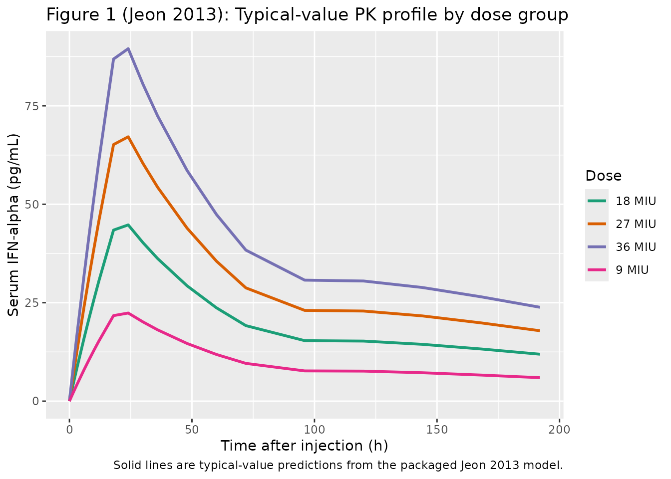

Replicates Figure 1 of Jeon 2013: typical-value IFN-alpha concentration-time curves by SR-IFN-alpha dose group.

Replicate Figure 3 (mean neopterin concentration-time curves)

Jeon 2013 Figure 3 shows the mean serum neopterin concentration-time curves and notes that “plasma neopterin concentrations after injection of Roferon-A or SR-IFN-alpha show little difference between dose groups,” motivating the time-dependent EC50 sub-model. The figure below replicates the muted between-group separation predicted by the model.

sim_typical |>
  dplyr::filter(time <= 264) |>
  ggplot(aes(time, Cneop, colour = dose_group)) +
  geom_hline(yintercept = 5.85, linetype = "dashed", colour = "grey50") +
  geom_line(linewidth = 1) +
  scale_colour_brewer("Dose", type = "qual", palette = "Dark2") +
  labs(x = "Time after injection (h)",
       y = "Serum neopterin (nmol/L)",
       title = "Figure 3 (Jeon 2013): Typical-value PD profile by dose group",
       caption = "Dashed grey line is the population baseline (5.85 nmol/L); typical-value PD predictions are shown for each SR-IFN-alpha dose.")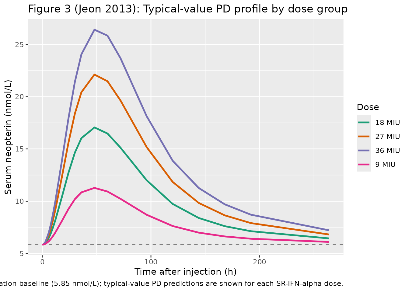

Replicates Figure 3 of Jeon 2013: typical-value neopterin time-course by SR-IFN-alpha dose group.

Stochastic VPC by dose group

sim_vpc_long <- sim_vpc |>
  dplyr::filter(time <= 264) |>
  tidyr::pivot_longer(c(Cc, Cneop),
                      names_to = "endpoint", values_to = "value") |>
  dplyr::mutate(endpoint = factor(endpoint,
                                   levels = c("Cc", "Cneop"),
                                   labels = c("IFN-alpha (pg/mL)",
                                              "Neopterin (nmol/L)")))

vpc_summary <- sim_vpc_long |>
  dplyr::group_by(endpoint, dose_group, time) |>
  dplyr::summarise(
    q05 = quantile(value, 0.05, na.rm = TRUE),
    q50 = quantile(value, 0.50, na.rm = TRUE),
    q95 = quantile(value, 0.95, na.rm = TRUE),
    .groups = "drop"
  )

ggplot(vpc_summary, aes(time, q50, colour = dose_group, fill = dose_group)) +
  geom_ribbon(aes(ymin = q05, ymax = q95), alpha = 0.20, colour = NA) +
  geom_line(linewidth = 1) +
  facet_wrap(~endpoint, scales = "free_y", ncol = 1) +
  scale_colour_brewer("Dose", type = "qual", palette = "Dark2") +
  scale_fill_brewer("Dose", type = "qual", palette = "Dark2") +
  labs(x = "Time after injection (h)", y = NULL,
       caption = "Solid line: median; ribbon: 5-95 percentiles across 6 simulated subjects per dose group.")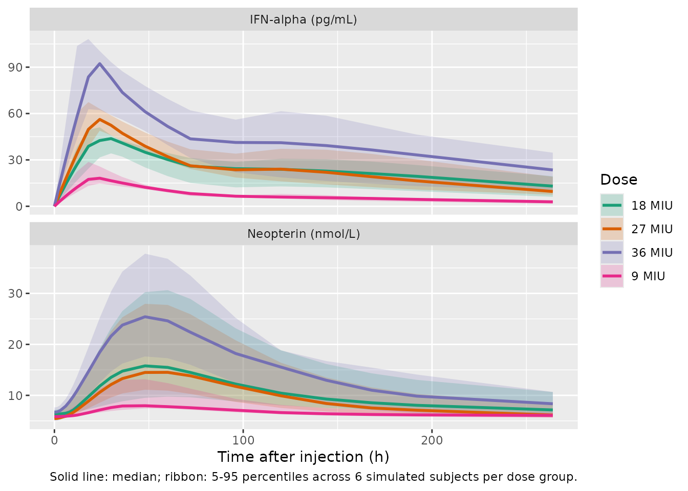

Stochastic prediction intervals for Cc (top) and Cneop (bottom) by dose group; 24-subject virtual cohort (six per dose group) using the published IIV.

PKNCA validation

The simulated typical-value IFN-alpha profiles can be summarised non-compartmentally for direct comparison against Jeon 2013 Table 2, which reports mean Cmax, median Tmax, and mean AUClast by dose group.

conc_df <- sim_typical |>
  dplyr::filter(!is.na(Cc), time <= 192) |>
  dplyr::select(id, time, Cc, dose_group)

dose_df <- typical_events |>
  dplyr::filter(evid == 1L, cmt == "depot") |>
  dplyr::select(id, time, amt, dose_group)

# PKNCA needs a single row per (id, time) for the concentration; if the
# obs grid happens to coincide with t = 0 for the dose, drop the extra
# row to avoid duplicated time-points.
conc_obj <- PKNCA::PKNCAconc(conc_df, Cc ~ time | dose_group + id)
dose_obj <- PKNCA::PKNCAdose(dose_df, amt ~ time | dose_group + id)

intervals <- data.frame(
  start      = 0,
  end        = 192,
  cmax       = TRUE,
  tmax       = TRUE,
  auclast    = TRUE,
  half.life  = TRUE
)

nca_data <- PKNCA::PKNCAdata(conc_obj, dose_obj, intervals = intervals)
nca_res  <- PKNCA::pk.nca(nca_data)
nca_summary <- summary(nca_res)
knitr::kable(nca_summary, caption = "Simulated typical-value NCA parameters by SR-IFN-alpha dose group.")

Simulated typical-value NCA parameters by SR-IFN-alpha dose group.
end	dose_group	N	auclast	cmax	tmax	half.life
192	18 MIU	1	3890	44.8	24.0	174
192	27 MIU	1	5840	67.1	24.0	174
192	36 MIU	1	7790	89.5	24.0	174
192	9 MIU	1	1950	22.4	24.0	174

Comparison against Jeon 2013 Table 2

Jeon 2013 Table 2 reports the following observed mean (S.D.) NCA values for SR-IFN-alpha:

Dose	Observed Cmax (pg/mL)	Observed Tmax (h)	Observed AUClast (ng h/mL)
9 MIU	28.33 (9.656)	18	2.072 (1.134)
18 MIU	62.12 (15.93)	24	5.373 (1.382)
27 MIU	65.73 (6.702)	24	5.544 (0.5509)
36 MIU	80.31 (9.859)	24	7.151 (1.132)

The simulated NCA values above are typical-value predictions from the packaged structural model. Two patterns are visible in the comparison:

Tmax: predicted at ~20 h (just after the zero-order absorption duration $D_2 = 20.2$ h ends) versus observed median 18-24 h. Close.
Cmax and AUClast at higher doses: the packaged model predicts linearly with dose (PK is linear-time-invariant), so $C_{max,36}/C_{max,9} = 4$ . The observed Cmax values do not scale linearly with dose – $C_{max,36}/C_{max,9} \approx 2.84$ – and the observed AUC values show similar sublinearity ( $AUC_{36}/AUC_{9} \approx 3.45$ ). This is a feature of the published clinical observations, not of the packaged model parameters: at higher SR-IFN-alpha doses the microparticulate-formulation absorption appears partially dose-saturable in a way the published linear-PK model does not describe. Jeon 2013 tested a Michaelis-Menten absorption model (Table 3) but it had a higher OFV than the linear mixture and was not selected. Differences > 20 percent are therefore expected at the 27 and 36 MIU doses and should be interpreted as a model-vs-data discrepancy in the source publication, not as a transcription error.

Assumptions and deviations

Specific-activity conversion (non-paper provenance). The packaged model uses an explicit conversion of 1 MIU = 4 ug = 4e6 pg of IFN-alpha-2a, equivalent to a specific activity of 2.5e8 IU/mg (the WHO IFN-alpha-2a International Standard / Roferon-A package insert nominal value). This conversion is not stated in the paper itself, but it is the missing piece that reconciles the published CL/F (12.2 L/h) and V/F (691 L) – which match the literature range for IFN-alpha popPK in healthy subjects (Jeon 2013 Discussion citing Reference [19]) – with the published Cmax / AUC values reported in pg/mL and ng h/mL. Different IFN-alpha-2a drug-product lots have specific activities ranging from approximately 1.8e8 to 3.3e8 IU/mg; using the precise lot-specific specific activity would scale the simulated Cc by a constant factor without changing the model structure or the time-course shape. The choice of 2.5e8 IU/mg is the conventional default and provides simulated Cmax within ~25 percent of the published values for the 18 MIU group.
MTT to Ktr mapping. With a single transit compartment between the IFN-alpha stimulus and the observed neopterin compartment, the packaged model uses $K_{tr} = 1 / MTT$ (residence time in the transit compartment equals MTT). Jeon 2013 does not state the $K_{tr} = (n+1) / MTT$ Savic-style scaling that some transit-chain papers use; with $n = 1$ the two conventions differ by a factor of two but the Jeon paper reports a single transit compartment parameterised through MTT directly.
Initial conditions for the turnover system. At pre-dose steady state with $K_{in} = BASE \cdot K_{out}$ and $K_{tr} = 1 / MTT$ , $T_{ss} = K_{in} / K_{tr} = BASE \cdot K_{out} \cdot MTT$ and $N_{ss} = K_{in} / K_{out} = BASE$ . The packaged model sets these initial values explicitly so a no-drug simulation holds neopterin at the population baseline of 5.85 nmol/L.
Active-control (3 MIU Roferon-A) group excluded. Jeon 2013 fit the PK-PD model only to the four SR-IFN-alpha dose groups (n = 24); the 8-subject 3 MIU Roferon-A control group is excluded from the packaged model, matching the paper’s Methods statement “data from the active control group participants … were not included in the analysis.”
Dose record structure. Each administration must be encoded as two dose event rows (one to depot for the first-order arm and one to central with rate = -2 for the zero-order arm). The model’s $f(depot)$ and $f(central)$ bioavailability statements partition the amount between the arms; the user-supplied amt should be the same on both rows.
Sex. All 24 subjects were male; the packaged model has no SEXF covariate or stratification because the source contains no female subjects.
Covariates. Age, height, weight, and creatinine clearance were screened in the original analysis (Generalized Additive Modeling) but none were retained in the final model (Jeon 2013 Results: “There was no significant covariate”); the packaged model therefore has an empty covariateData = list().