Bedaquiline (Shao 2023)
Source:vignettes/articles/Shao_2023_bedaquiline.Rmd
Shao_2023_bedaquiline.RmdModel and source
- Citation: Shao G, Bao Z, Davies Forsman L, Paues J, Werngren J, Niward K, Schon T, Bruchfeld J, Alffenaar J-W, Hu Y (2023). Population pharmacokinetics and model-based dosing evaluation of bedaquiline in multidrug-resistant tuberculosis patients. Frontiers in Pharmacology 14:1022090. doi:10.3389/fphar.2023.1022090. The absorption sub-model constants (Ka fixed at 1,000 1/h, DUR1 = 2.22 h, DUR2 = 1.48 h and FR1 = 58.5%) were fixed by Shao 2023 from McLeay SC, Vis P, van Heeswijk RPG, Green B (2014), Population pharmacokinetics of bedaquiline (TMC207), a novel antituberculosis drug, Antimicrobial Agents and Chemotherapy 58(9):5315-5324, doi:10.1128/AAC.01418-13; every one of those values is reprinted in Shao 2023 Methods section 2.2 and Table 2, so no value in this file is taken from the McLeay paper itself.
- Description: Three-compartment population PK model for bedaquiline in adult Chinese patients with multidrug-resistant tuberculosis (MDR-TB), with the dual zero-order absorption input of McLeay 2014 that reproduces the double absorption peak: a fixed fraction FR1 = 58.5% of the dose enters a depot compartment as a zero-order infusion of duration DUR1 = 2.22 h beginning after a lag of 1.00 h, and is then handed to the central compartment by a near-instantaneous first-order step (Ka fixed at 1,000 1/h), while the remaining 41.5% enters the central compartment directly as a zero-order infusion of duration DUR2 = 1.48 h beginning after an additional lag of 2.76 h (total 3.76 h). Apparent clearance CL/F is scaled by body weight with the allometric exponent fixed at 0.75 and by a steep power function of serum albumin with an estimated exponent of 3.76; apparent central volume Vc/F is scaled by body weight with the exponent fixed at 1. Both covariates are normalised to the development-cohort medians of 67 kg and 37.1 g/L. Between-subject variability is carried on CL/F and Vc/F and the residual error is proportional.
- Article: https://doi.org/10.3389/fphar.2023.1022090
Shao and colleagues fitted a three-compartment population PK model with a dual zero-order absorption input to richly-sampled bedaquiline concentrations from 55 Chinese adults treated for multidrug-resistant tuberculosis (MDR-TB), then used the model to estimate exposure in a separate prospective validation cohort of 159 patients, derived AUC0-24h/MIC thresholds predictive of sputum culture conversion by classification and regression tree (CART) analysis, and evaluated the WHO recommended dosing regimen by probability of target attainment (PTA).
Only the population PK model is packaged here. The CART thresholds (AUC0-24h/MIC of 175.5, 118.2 and 74.6) are not model parameters – they are outputs of a downstream statistical analysis – but they are used below to replicate the paper’s PTA analysis, which is a simulation from this model.
mod <- readModelDb("Shao_2023_bedaquiline")
ui  <- rxode2::rxode(mod)
#> ℹ parameter labels from comments will be replaced by 'label()'
Population
The model was fitted to the development cohort: 55 adults with MDR-TB enrolled in a multi-centre prospective cohort study across Guizhou, Henan, Jiangsu and Sichuan Provinces in China between June 2016 and June 2019 (Shao 2023 Methods 2.1). Median (IQR) age was 44 (34, 53) years, 39 of 55 (70.9%) were male, median (IQR) weight was 67 (59, 74) kg, median (IQR) height 165 (158, 173) cm, and median (IQR) serum albumin 37.1 (32.0, 40.6) g/L (Shao 2023 Table 1). Patients with abnormal liver or kidney function, pregnancy, or HIV / hepatitis B / hepatitis C infection were excluded. Plasma was drawn predose and at 1, 2, 3, 4, 5, 6, 8, 12, 18 and 24 h after dosing on treatment weeks 2 and 4, yielding 1,205 quantifiable concentrations spanning 0.04-5.96 mg/L; five samples below the 10 ng/mL LLOQ were discarded (Shao 2023 Results 3.2).
All participants received the WHO recommended bedaquiline regimen – 400 mg once daily for the first 2 weeks, then 200 mg three times weekly for the following 22 weeks – inside a standardised bedaquiline-containing MDR-TB regimen.
The separate validation cohort of 159 MDR-TB patients (median weight 65 kg, median albumin 37.2 g/L, sparse sampling predose and at 2, 4 and 6 h on week 4) was not used to estimate the parameters packaged here; it was used only for Bayesian post-hoc exposure estimation, CART threshold derivation and the PTA analysis. Because every published exposure number (AUC0-24h, Cmax, Cmin, PTA) comes from that validation cohort, the virtual cohort below is built to the validation cohort’s demographics.
The same information is available programmatically via
readModelDb("Shao_2023_bedaquiline")()$population.
Source trace
The per-parameter origin is recorded as an in-file comment next to
each ini() entry in
inst/modeldb/specificDrugs/Shao_2023_bedaquiline.R. The
table below collects them in one place for review.
| Equation / parameter | Value | Source location |
|---|---|---|
lcl (CL/F) |
3.57 L/h | Table 2, “CL/F (L/h)” (RSE 11.9%, 95% CI 2.73-4.40) |
lvc (Vc/F) |
336.97 L | Table 2, “Vc/F (L)” (RSE 12.6%, 95% CI 253.86-420.08) |
lvp (Vp1/F) |
2839.13 L | Table 2, “Vp1/F (L)” (RSE 46.3%) |
lq (CLp1/F) |
2.97 L/h | Table 2, “CLp1/F (L/h)” (RSE 41.40%) |
lvp2 (Vp2/F) |
1391.89 L | Table 2, “Vp2/F (L)” (RSE 37.41%) |
lq2 (CLp2/F) |
9.81 L/h | Table 2, “CLp2/F (L/h)” (RSE 18.86%) |
lka (Ka) |
1000 1/h, fixed | Methods 2.2, “we fixed the absorption rate as 1,000 h-1 based on a published population PK model (McLeay et al., 2014)” |
lfdepot (FR1) |
0.585, fixed | Table 2, “FR1 (%)” = 58.5 (no RSE / CI); Methods 2.2 |
ld1 (DUR1) |
2.22 h, fixed | Table 2, “DUR1 (h)” (no RSE / CI); Methods 2.2 |
ld2 (DUR2) |
1.48 h, fixed | Table 2, “DUR2 (h)” (no RSE / CI); Methods 2.2 |
ltlag (Tlag) |
1.00 h | Table 2, “Tlag (h)” (RSE 9.1%, 95% CI 0.82-1.18) |
ltlag_add (Tlag,add) |
2.76 h | Table 2, “Tlag, add (h)” (RSE 21.0%, 95% CI 1.62-3.90) |
e_wt_cl |
0.75, fixed | Table 2, “Weight effect on CL”; Results 3.2 (allometric) |
e_wt_vc |
1, fixed | Table 2, “Weight effect on Vc”; Results 3.2 (allometric) |
e_alb_cl |
3.76 | Table 2, “Albumin effect on CL” (RSE 14.2%, 95% CI 2.71-4.80); Eq. 5 |
etalvc |
omega^2 = 0.38 | Table 2, “omega^2 V” (RSE 67.99%) |
etalcl |
omega^2 = 1.33 | Table 2, “omega^2 CL” (RSE 166.76%) |
propSd |
sqrt(0.23) = 0.4796 | Table 2 residual variance 0.23 (RSE 2.75%, 95% CI 0.22-0.24); Results 3.2, “A proportional error model was used” |
IIV form theta_i = theta_TV * exp(eta_i)
|
n/a | Eq. 1 |
Covariate form
theta_i = theta_TV * (cov_i / cov_median)^theta_cov
|
n/a | Eq. 2 |
vc <- 336.97 * (WT / 67)^1 |
n/a | Eq. 4 |
cl <- 3.57 * (WT / 67)^0.75 * (ALB / 37.1)^3.76 |
n/a | Eq. 5 |
| Weight centring constant 67 kg | n/a | Eq. 4, Eq. 5, and the sentence after Eq. 5 (“The median weight was 67 kg”); Table 1 development cohort |
| Albumin centring constant 37.1 g/L | n/a | Eq. 5 and the sentence after Eq. 5; Table 1 development cohort |
| Three-compartment disposition with dual zero-order input | n/a | Results 3.2 (“best described by a three-compartment model with dual zero-order input”) |
Dose split: FR1 to depot over DUR1, 1-FR1 to
central over DUR2 |
n/a | Methods 2.2; Table 2 footnote (FR1 / DUR1 / DUR2 definitions) |
| Second-arm lag = Tlag + Tlag,add | n/a | Table 2 footnote, “Tlag, add, Additional lag time prior to administration of the remaining dose into Vc/F” |
| CART thresholds 175.5 / 118.2 / 74.6 (used for PTA only) | n/a | Results 3.3, Figure 5 |
| PTA target regimens | n/a | Methods 2.4, Results 3.4, Figure 7 |
Structural check: the dual zero-order absorption input
The distinguishing feature of this model is the absorption sub-model. A single oral administration is delivered as two zero-order inputs:
- fraction
FR1= 58.5% entersdepotas a zero-order infusion of durationDUR1= 2.22 h beginning atTlag= 1.00 h, and is handed on tocentralby a first-order step withKafixed at 1,000 1/h (a depot half-life of 0.0007 h, i.e. effectively instantaneous – exactly what Shao 2023 Methods 2.2 intends by “the dose via the input compartment describing an initial zero-order (rather than first-order) input”); - the remaining 41.5% enters
centraldirectly as a zero-order infusion of durationDUR2= 1.48 h beginning atTlag + Tlag,add= 3.76 h.
Because the first arm finishes at 1.00 + 2.22 = 3.22 h and the second
does not start until 3.76 h, there is a 0.54 h window with no input at
all. That gap is what produces the double absorption peak Shao 2023
gives as the reason for choosing this structure (Results 3.2, “to
capture dual peaks observed during absorption”). Each administration
therefore needs two dose records in the event table –
one to depot, one to central, each carrying
the whole dose (the f() multipliers do the FR1
split) and each carrying its zero-order duration explicitly in a
dur column. The model declares those same durations as
dur(depot) <- d1 / dur(central) <- d2;
see the chunk below for why the event table states them rather than
requesting them with rate = -2.
# Two dose records per administration, each carrying its zero-order duration
# explicitly in a `dur` column rather than via `rate = -2`.
#
# The model still declares `dur(depot) <- d1` / `dur(central) <- d2`, and the
# two forms are numerically identical here (max |dCc| = 1.1e-16 over the
# profile) because DUR1 and DUR2 are `fixed()` constants -- 2.22 h and 1.48 h,
# Shao 2023 Table 2 -- carrying no eta and no covariate, so the modelled
# duration cannot vary by subject.
#
# The explicit column is used because the RELEASED rxode2 (5.1.6) cannot solve
# TWO SIMULTANEOUS modelled-duration doses into different compartments: this
# dual zero-order input is exactly that shape, and it fails with "could not
# solve the system" (Data error 686/886). One such dose is fine, and an
# explicit `dur` is fine; only the pair fails. It is tolerated on the
# unreleased 5.1.7, so writing `rate = -2` renders locally and breaks CI.
DUR1 <- 2.22   # Shao 2023 Table 2, fixed
DUR2 <- 1.48   # Shao 2023 Table 2, fixed
doseRecords <- function(id, times, amt) {
  dplyr::bind_rows(
    tibble(id = id, time = times, amt = amt, cmt = "depot",
           evid = 1L, dur = DUR1),
    tibble(id = id, time = times, amt = amt, cmt = "central",
           evid = 1L, dur = DUR2)
  )
}

# Observation rows target the ODE state `central`, never the algebraic
# observable `Cc`; rxode2 returns Cc as a column regardless.
obsRecords <- function(id, times) {
  tibble(id = id, time = times, amt = NA_real_, cmt = "central",
         evid = 0L, dur = NA_real_)
}

evSingle <- dplyr::bind_rows(
  doseRecords(1L, 0, 400),
  obsRecords(1L, seq(0, 12, by = 0.01))
) |>
  dplyr::mutate(WT = 67, ALB = 37.1) |>
  dplyr::arrange(id, time, dplyr::desc(evid))

# Typical-value solve: zeroRe() blanks the random effects and omega = NA stops
# rxSolve from re-using a previously attached omega.
simSingle <- rxode2::rxSolve(
  rxode2::zeroRe(mod), evSingle, omega = NA,
  returnType = "data.frame", addDosing = FALSE
)
#> ℹ parameter labels from comments will be replaced by 'label()'
cc <- simSingle$Cc
tt <- simSingle$time
localMax <- tt[which(diff(sign(diff(cc))) < 0) + 1]
localMin <- tt[which(diff(sign(diff(cc))) > 0) + 1]

# Look concentrations up by NEAREST grid point, never by `tt == target`.
# `seq(0, 12, by = 0.01)` accumulates floating-point error, so e.g. the element
# that prints as 3.76 is actually 3.7600000000000002 and `tt == 3.76` matches
# nothing -- silently yielding a zero-length vector rather than an error.
ccAt <- function(target) cc[which.min(abs(tt - target))]

# The turning points are structural identities of the absorption sub-model,
# not fitted quantities, so they can be asserted exactly (to the resolution of
# the 0.01 h observation grid):
#   peak 1   at Tlag + DUR1              = 1.00 + 2.22            = 3.22 h
#   trough   at Tlag + Tlag,add          = 1.00 + 2.76            = 3.76 h
#   peak 2   at Tlag + Tlag,add + DUR2   = 1.00 + 2.76 + 1.48     = 5.24 h
stopifnot(
  length(localMax) == 2L,
  isTRUE(all.equal(localMax, c(3.22, 5.24), tolerance = 1e-6)),
  # The first "minimum" is the flat pre-lag stretch at Cc = 0; the informative
  # one is the input gap.
  any(abs(localMin - 3.76) < 1e-6)
)

tibble(
  Feature  = c("Peak 1 (end of depot arm)", "Trough (input gap)",
               "Peak 2 (end of central arm)"),
  `Predicted time (h)` = c(1.00 + 2.22, 1.00 + 2.76, 1.00 + 2.76 + 1.48),
  `Simulated time (h)` = c(localMax[1], 3.76, localMax[2]),
  `Cc (mg/L)` = c(ccAt(localMax[1]), ccAt(3.76), ccAt(localMax[2]))
) |>
  knitr::kable(digits = 4,
caption = "Turning points of the dual zero-order input after a single 400 mg dose (typical subject, 67 kg, 37.1 g/L).")| Feature | Predicted time (h) | Simulated time (h) | Cc (mg/L) |
|---|---|---|---|
| Peak 1 (end of depot arm) | 3.22 | 3.22 | 0.6582 |
| Trough (input gap) | 3.76 | 3.76 | 0.6416 |
| Peak 2 (end of central arm) | 5.24 | 5.24 | 1.0730 |
ggplot(simSingle, aes(time, Cc)) +
  geom_line(linewidth = 0.7) +
  geom_vline(xintercept = c(1.00, 3.22, 3.76, 5.24),
             linetype = "dashed", colour = "grey55") +
  annotate("text", x = c(1.00, 3.22, 3.76, 5.24), y = max(cc) * 1.04,
           label = c("Tlag", "end DUR1", "start arm 2", "end DUR2"),
           size = 2.8, hjust = -0.05) +
  coord_cartesian(ylim = c(0, max(cc) * 1.12)) +
  labs(x = "Time after a single 400 mg dose (h)", y = "Cc (mg/L)",
       title = "Dual zero-order absorption input",
       caption = paste("Reproduces the absorption phase Shao 2023 Results 3.2",
                       "describes as 'dual peaks observed during absorption'."))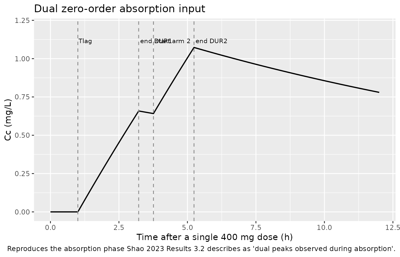
Structural check: the covariate model reproduces Eq. 4 and Eq. 5
cl and vc are returned by
rxSolve() as columns, so the published equations can be
checked directly rather than by eye.
covCheck <- tibble(
  id  = 1:4,
  WT  = c(67, 50, 90, 67),
  ALB = c(37.1, 37.1, 37.1, 30)
)

evCov <- dplyr::bind_rows(lapply(covCheck$id, function(i) {
  dplyr::bind_rows(doseRecords(i, 0, 400), obsRecords(i, c(0, 24)))
})) |>
  dplyr::left_join(covCheck, by = "id") |>
  dplyr::arrange(id, time, dplyr::desc(evid))

simCov <- rxode2::rxSolve(
  rxode2::zeroRe(mod), evCov, omega = NA,
  returnType = "data.frame", addDosing = FALSE
) |>
  dplyr::distinct(id, cl, vc) |>
  dplyr::left_join(covCheck, by = "id") |>
  dplyr::mutate(
    # Shao 2023 Eq. 5 and Eq. 4, typed out independently of the model file.
    cl_eq5 = 3.57   * (WT / 67)^0.75 * (ALB / 37.1)^3.76,
    vc_eq4 = 336.97 * (WT / 67)^1
  )
#> ℹ parameter labels from comments will be replaced by 'label()'
#> Warning: multi-subject simulation without without 'omega'

stopifnot(
  isTRUE(all.equal(simCov$cl, simCov$cl_eq5, tolerance = 1e-8)),
  isTRUE(all.equal(simCov$vc, simCov$vc_eq4, tolerance = 1e-8)),
  # At the reference covariates the published typical values must come back
  # exactly.
  isTRUE(all.equal(simCov$cl[simCov$WT == 67 & simCov$ALB == 37.1][1], 3.57,
                   tolerance = 1e-10)),
  isTRUE(all.equal(simCov$vc[simCov$WT == 67][1], 336.97, tolerance = 1e-10))
)

simCov |>
  dplyr::select(WT, ALB, cl, cl_eq5, vc, vc_eq4) |>
  dplyr::rename(
    "WT (kg)"          = WT,
    "ALB (g/L)"        = ALB,
    "CL/F model (L/h)" = cl,
    "CL/F Eq. 5 (L/h)" = cl_eq5,
    "Vc/F model (L)"   = vc,
    "Vc/F Eq. 4 (L)"   = vc_eq4
  ) |>
  knitr::kable(digits = 4,
caption = "The packaged model reproduces Shao 2023 Eq. 4 and Eq. 5 exactly.")| WT (kg) | ALB (g/L) | CL/F model (L/h) | CL/F Eq. 5 (L/h) | Vc/F model (L) | Vc/F Eq. 4 (L) |
|---|---|---|---|---|---|
| 67 | 37.1 | 3.5700 | 3.5700 | 336.9700 | 336.9700 |
| 50 | 37.1 | 2.8664 | 2.8664 | 251.4701 | 251.4701 |
| 90 | 37.1 | 4.4544 | 4.4544 | 452.6463 | 452.6463 |
| 67 | 30.0 | 1.6062 | 1.6062 | 336.9700 | 336.9700 |
The albumin exponent is steep. Across the development cohort’s albumin IQR (32.0-40.6 g/L) the multiplier on CL/F spans 0.573 to 1.403, a 2.45-fold range – larger than the effect of body weight over the same cohort.
Virtual cohort
Original observed data are not publicly available. The cohort below approximates the validation cohort demographics (Shao 2023 Table 1: median weight 65 kg, IQR 59-71; median albumin 37.2 g/L, IQR 32.4-41.6), because every published exposure and PTA number comes from that cohort.
Between-subject variability is drawn in R with
set.seed() and passed to rxSolve() as
event-table columns (etalcl,
etalvc) with omega = NA, rather than being
sampled by rxode2. rxode2 partitions its RNG stream per solver thread,
so a cohort it samples is not reproducible across machines with
different thread counts; drawing the etas in base R makes every number
on this page identical on any machine. Note that Cc is the
individual prediction and carries no residual error, so
the spread below is between-subject variability only.
set.seed(1022090)

nPerArm <- 200L  # cap is 200 participants per arm

# Log-normal covariate draws whose medians and IQRs match Shao 2023 Table 1
# (validation cohort). sdlog is back-solved from the reported quartiles:
#   WT : log(71 / 65)   / qnorm(0.75) = 0.130
#   ALB: log(41.6 / 37.2)/ qnorm(0.75) = 0.166 and
#        log(37.2 / 32.4)/ qnorm(0.75) = 0.205 -> 0.185 used (their average)
subjects <- tibble(
  subj    = seq_len(nPerArm),
  WT      = exp(rnorm(nPerArm, log(65),   0.130)),
  ALB     = exp(rnorm(nPerArm, log(37.2), 0.185)),
  etalcl  = rnorm(nPerArm, 0, sqrt(1.33)),   # Shao 2023 Table 2 omega^2 CL
  etalvc  = rnorm(nPerArm, 0, sqrt(0.38))    # Shao 2023 Table 2 omega^2 V
)

# --- The three regimens Shao 2023 evaluates (Methods 2.4) ---------------
# A. WHO recommended: 400 mg QD x 14 d, then 200 mg thrice weekly (Mon/Wed/Fri).
#    AUC0-24h taken on treatment week 4.
# B. 200 mg once daily. AUC0-24h taken on treatment week 4.
# C. 200 mg once daily x 56 d, then 100 mg once daily. AUC0-24h on week 10.
day <- function(d) (d - 1) * 24          # hour of the dose on treatment day d
whoMaintDays <- c(seq(15, 19, by = 2), seq(22, 26, by = 2))  # Mon/Wed/Fri, wk 3-4

regimens <- list(
  list(name    = "A. WHO 400 mg QD x14d then 200 mg TIW",
       doses   = dplyr::bind_rows(
         tibble(time = day(1:14),           amt = 400),
         tibble(time = day(whoMaintDays),   amt = 200)),
       ncaStart = day(22),                 # first week-4 dose
       ncaWeek  = "week 4"),
  list(name    = "B. 200 mg QD",
       doses   = tibble(time = day(1:28), amt = 200),
       ncaStart = day(22),
       ncaWeek  = "week 4"),
  list(name    = "C. 200 mg QD x56d then 100 mg QD",
       doses   = dplyr::bind_rows(
         tibble(time = day(1:56),  amt = 200),
         tibble(time = day(57:70), amt = 100)),
       ncaStart = day(66),                 # a week-10 dose
       ncaWeek  = "week 10")
)

buildArm <- function(reg, idOffset) {
  ids <- idOffset + subjects$subj
  dos <- dplyr::bind_rows(lapply(seq_along(ids), function(k)
    doseRecords(ids[k], reg$doses$time, reg$doses$amt)))
  # Coarse grid for accumulation, dense grid over the NCA interval.
  coarse <- seq(0, reg$ncaStart, by = 12)
  dense  <- seq(reg$ncaStart, reg$ncaStart + 24, by = 0.25)
  obsT   <- sort(unique(c(coarse, dense)))
  obs <- dplyr::bind_rows(lapply(ids, function(i) obsRecords(i, obsT)))
  dplyr::bind_rows(dos, obs) |>
    dplyr::mutate(subj = .data$id - idOffset) |>
    dplyr::left_join(subjects, by = "subj") |>
    dplyr::mutate(treatment = reg$name, ncaStart = reg$ncaStart) |>
    dplyr::select(-subj) |>
    dplyr::arrange(.data$id, .data$time, dplyr::desc(.data$evid))
}

events <- dplyr::bind_rows(
  buildArm(regimens[[1]],       0L),
  buildArm(regimens[[2]], 1000L),
  buildArm(regimens[[3]], 2000L)
)

# Disjoint IDs across arms are mandatory: rxSolve treats id as the subject key
# and silently merges duplicates into a single subject receiving the summed dose.
stopifnot(!anyDuplicated(unique(events[, c("id", "time", "evid")])))
Simulation
sim <- rxode2::rxSolve(
  mod, events = events, omega = NA,
  keep = c("treatment", "ncaStart", "WT", "ALB"),
  returnType = "data.frame", addDosing = FALSE
)
#> ℹ parameter labels from comments will be replaced by 'label()'
#> Warning: multi-subject simulation without without 'omega'

# Two independent properties are gated here.
#
# 1. The eta and covariate columns were actually CONSUMED. With 200 distinct
#    (etalcl, etalvc, WT, ALB) tuples the model must produce 200 distinct
#    clearances and volumes -- not one, which is what a silently-dropped
#    covariate column would give.
# 2. Common random numbers hold ACROSS arms. The same 200 subjects are reused
#    in all three regimens, so subject k has the identical cl and vc in each
#    arm and only the dosing differs. That is what makes the regimen A vs B
#    comparison below an exact per-subject contrast rather than a noisy
#    between-cohort one, so it is asserted rather than assumed.
stopifnot(
  dplyr::n_distinct(round(sim$cl, 8)) == nPerArm,
  dplyr::n_distinct(round(sim$vc, 8)) == nPerArm,
  dplyr::n_distinct(sim$treatment) == 3L
)

crn <- sim |>
  dplyr::distinct(id, treatment, cl, vc) |>
  dplyr::mutate(subj = id %% 1000L) |>
  dplyr::group_by(subj) |>
  dplyr::summarise(
    nArm = dplyr::n_distinct(treatment),
    nCl  = dplyr::n_distinct(round(cl, 10)),
    nVc  = dplyr::n_distinct(round(vc, 10)),
    .groups = "drop"
  )
stopifnot(
  nrow(crn) == nPerArm,
  all(crn$nArm == 3L),
  all(crn$nCl == 1L),
  all(crn$nVc == 1L)
)
Replicate published figures
Concentration-time profile over the week-4 dosing interval
Shao 2023 Figure 3C is a visual predictive check of the final model over the week-4 dosing interval in the validation cohort. The observed concentrations are not public, so the panel below shows the simulated 5th / 50th / 95th percentiles alone, on the same interval and the same regimen.
whoName <- regimens[[1]]$name

sim |>
  dplyr::filter(treatment == whoName,
                time >= ncaStart, time <= ncaStart + 24) |>
  dplyr::mutate(tad = time - ncaStart) |>
  dplyr::group_by(tad) |>
  dplyr::summarise(
    Q05 = quantile(Cc, 0.05), Q50 = quantile(Cc, 0.50),
    Q95 = quantile(Cc, 0.95), .groups = "drop"
  ) |>
  ggplot(aes(tad, Q50)) +
  geom_ribbon(aes(ymin = Q05, ymax = Q95), alpha = 0.25) +
  geom_line(linewidth = 0.7) +
  scale_y_log10() +
  labs(x = "Time after dose (h)", y = "Cc (mg/L, log scale)",
       title = "Week-4 dosing interval, WHO recommended regimen",
       caption = paste("Structure of Figure 3C of Shao 2023 (simulated",
                       "percentiles only; observed data are not public)."))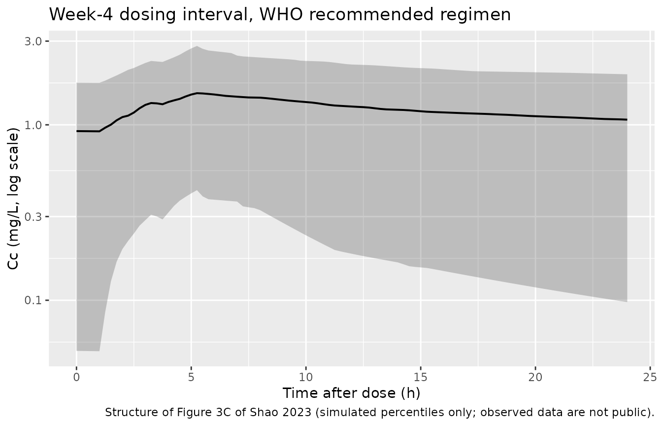
Exposure accumulation over the first four weeks
sim |>
  dplyr::filter(treatment == whoName, time <= regimens[[1]]$ncaStart + 24) |>
  dplyr::group_by(time) |>
  dplyr::summarise(
    Q05 = quantile(Cc, 0.05), Q50 = quantile(Cc, 0.50),
    Q95 = quantile(Cc, 0.95), .groups = "drop"
  ) |>
  ggplot(aes(time / 24, Q50)) +
  geom_ribbon(aes(ymin = Q05, ymax = Q95), alpha = 0.25) +
  geom_line(linewidth = 0.7) +
  geom_vline(xintercept = 14, linetype = "dashed", colour = "grey55") +
  labs(x = "Treatment day", y = "Cc (mg/L)",
       title = "Loading phase (400 mg QD) then maintenance (200 mg TIW)",
       caption = paste("Dashed line marks the end of the 2-week loading",
                       "phase. Median with 5th-95th percentile band."))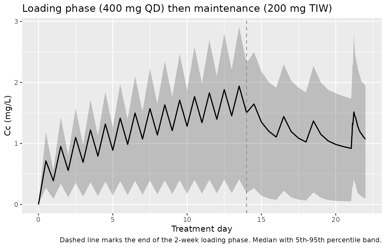
PKNCA validation
NCA is run on each arm’s target dosing interval, with time re-anchored to zero at that interval’s dose so the interval definition is identical across arms.
ncaConc <- sim |>
  dplyr::filter(!is.na(Cc), time >= ncaStart, time <= ncaStart + 24) |>
  dplyr::mutate(time = time - ncaStart) |>
  dplyr::select(id, time, Cc, treatment)

# Time-zero guarantee: the dose time is already on the grid, so this is a
# no-op here, but it is kept as a defensive step (PKNCA warns loudly if the
# AUC interval starts before the first measurement).
ncaConc <- dplyr::bind_rows(
  ncaConc,
  ncaConc |> dplyr::distinct(id, treatment) |>
    dplyr::mutate(time = 0, Cc = NA_real_)
) |>
  dplyr::arrange(id, treatment, time) |>
  dplyr::distinct(id, treatment, time, .keep_all = TRUE) |>
  dplyr::filter(!is.na(Cc))

ncaDose <- events |>
  dplyr::filter(evid == 1L, cmt == "central", time == ncaStart) |>
  dplyr::mutate(time = 0) |>
  dplyr::select(id, time, amt, treatment)

concObj <- PKNCA::PKNCAconc(ncaConc, Cc ~ time | treatment + id,
                            concu = "mg/L", timeu = "h")
doseObj <- PKNCA::PKNCAdose(ncaDose, amt ~ time | treatment + id,
                            doseu = "mg")

intervals <- data.frame(
  start   = 0,
  end     = 24,
  cmax    = TRUE,
  tmax    = TRUE,
  cmin    = TRUE,
  # `ctrough` (concentration at the interval end) is PKNCA's name for what a
  # NONMEM-era table would call Ctau; `ctau` is not a valid interval column.
  ctrough = TRUE,
  cav     = TRUE,
  auclast = TRUE
)

ncaRes <- PKNCA::pk.nca(
  PKNCA::PKNCAdata(concObj, doseObj, intervals = intervals)
)

ncaWide <- as.data.frame(ncaRes) |>
  dplyr::select(treatment, id, PPTESTCD, PPORRES) |>
  tidyr::pivot_wider(names_from = PPTESTCD, values_from = PPORRES)
Comparison against published NCA
Shao 2023 reports validation-cohort exposure on treatment week 4 in Results 3.3 (whole-cohort median AUC0-24h) and Table 3 (Cmax, Cmin and AUC0-24h split by treatment outcome). The reference row below takes AUC0-24h = 31.7 mg*h/L from the whole-cohort statement in Results 3.3, and Cmax = 1.8 mg/L and Cmin = 1.1 mg/L from the Table 3 “successful treatment outcome / negative” column, which covers 149 of the 159 patients (93.7%) and is therefore the closest thing the paper reports to a whole-cohort central value for those two parameters.
published <- tibble::tribble(
  ~treatment,  ~cmax, ~cmin, ~auclast,
  whoName,     1.8,   1.1,   31.7
)

cmp <- nlmixr2lib::ncaComparisonTable(
  simulated = ncaWide |> dplyr::filter(treatment == whoName),
  reference = published,
  by        = "treatment",
  params    = c("cmax", "cmin", "auclast"),
  units     = c(cmax = "mg/L", cmin = "mg/L", auclast = "mg*h/L"),
  tolerance_pct = 20
)

knitr::kable(
  cmp,
  caption = paste("Simulated (median of 200 virtual subjects) vs published",
                  "week-4 exposure, WHO recommended regimen.",
                  "* differs from reference by more than 20%."),
  align = c("l", "l", "r", "r", "r")
)| NCA parameter | treatment | Reference | Simulated | % diff |
|---|---|---|---|---|
| Cmax (mg/L) | A. WHO 400 mg QD x14d then 200 mg TIW | 1.8 | 1.51 | -15.9% |
| Cmin (mg/L) | A. WHO 400 mg QD x14d then 200 mg TIW | 1.1 | 0.918 | -16.5% |
| AUClast (mg*h/L) | A. WHO 400 mg QD x14d then 200 mg TIW | 31.7 | 29.4 | -7.2% |
ncaWide |>
  dplyr::group_by(treatment) |>
  dplyr::summarise(
    `AUC0-24h Q1`     = quantile(auclast, 0.25),
    `AUC0-24h median` = median(auclast),
    `AUC0-24h Q3`     = quantile(auclast, 0.75),
    `Cmax median`     = median(cmax),
    `Cmin median`     = median(cmin),
    `Ctrough median`  = median(ctrough),
    `Tmax median`     = median(tmax),
    .groups = "drop"
  ) |>
  dplyr::rename("Regimen" = treatment) |>
  knitr::kable(digits = 2,
caption = "Simulated NCA over the target dosing interval, by regimen (AUC in mg*h/L, concentrations in mg/L, times in h).")| Regimen | AUC0-24h Q1 | AUC0-24h median | AUC0-24h Q3 | Cmax median | Cmin median | Ctrough median | Tmax median |
|---|---|---|---|---|---|---|---|
| A. WHO 400 mg QD x14d then 200 mg TIW | 18.23 | 29.43 | 41.55 | 1.51 | 0.92 | 1.07 | 5.25 |
| B. 200 mg QD | 18.00 | 27.29 | 35.81 | 1.44 | 0.90 | 0.93 | 5.25 |
| C. 200 mg QD x56d then 100 mg QD | 14.89 | 29.96 | 51.89 | 1.45 | 1.13 | 1.13 | 5.25 |
whoAuc <- ncaWide$auclast[ncaWide$treatment == whoName]

# Structural / centre assertions only. The published 31.7 mg*h/L is the median
# of Bayesian post-hoc estimates in a different (sparsely sampled) cohort, so a
# forward simulation is not expected to land on it exactly; the gate is on the
# CENTRE with generous headroom, never on an extreme of a random cohort.
# Observed here: median 29.4 mg*h/L, i.e. 7% below the published median.
stopifnot(
  abs(median(whoAuc) / 31.7 - 1) < 0.30,
  # Interquartile spread of the same order as the published IQR (13.9, 48.5),
  # whose Q3/Q1 ratio is 3.5. Observed here: 2.3.
  quantile(whoAuc, 0.75) / quantile(whoAuc, 0.25) > 1.5,
  quantile(whoAuc, 0.75) / quantile(whoAuc, 0.25) < 8,
  # Tmax must land on the second absorption peak, not the first.
  median(ncaWide$tmax[ncaWide$treatment == whoName]) > 3.76
)
Replicate Figure 7: probability of target attainment
Shao 2023 Methods 2.4 and Results 3.4 evaluate the three regimens against the three CART-derived AUC0-24h/MIC thresholds across a 7H11 MIC distribution of 0.015-1 mg/L. The paper simulated 1,000 patients per regimen; the cap here is 200 per arm, which is ample for the percentages below.
mics    <- c(0.015, 0.03, 0.06, 0.125, 0.25, 0.5, 1)
targets <- c(`2-month conversion (175.5)` = 175.5,
             `6-month conversion (118.2)` = 118.2,
             `Successful outcome (74.6)`  = 74.6)

pta <- tidyr::expand_grid(
  treatment = unique(ncaWide$treatment),
  MIC       = mics,
  Target    = names(targets)
) |>
  dplyr::rowwise() |>
  dplyr::mutate(
    PTA = 100 * mean(
      ncaWide$auclast[ncaWide$treatment == treatment] / MIC > targets[[Target]]
    )
  ) |>
  dplyr::ungroup()

ggplot(pta, aes(factor(MIC), PTA, colour = treatment, group = treatment)) +
  geom_line() +
  geom_point(size = 1.5) +
  geom_hline(yintercept = 90, linetype = "dashed", colour = "grey40") +
  facet_wrap(~Target) +
  scale_y_continuous(limits = c(0, 100)) +
  theme(legend.position = "bottom", legend.direction = "vertical") +
  labs(x = "7H11 MIC (mg/L)", y = "Probability of target attainment (%)",
       colour = NULL,
       title = "Probability of target attainment by MIC and CART threshold",
       caption = paste("Replicates Figure 7 of Shao 2023. Dashed line is the",
                       "90% PTA criterion."))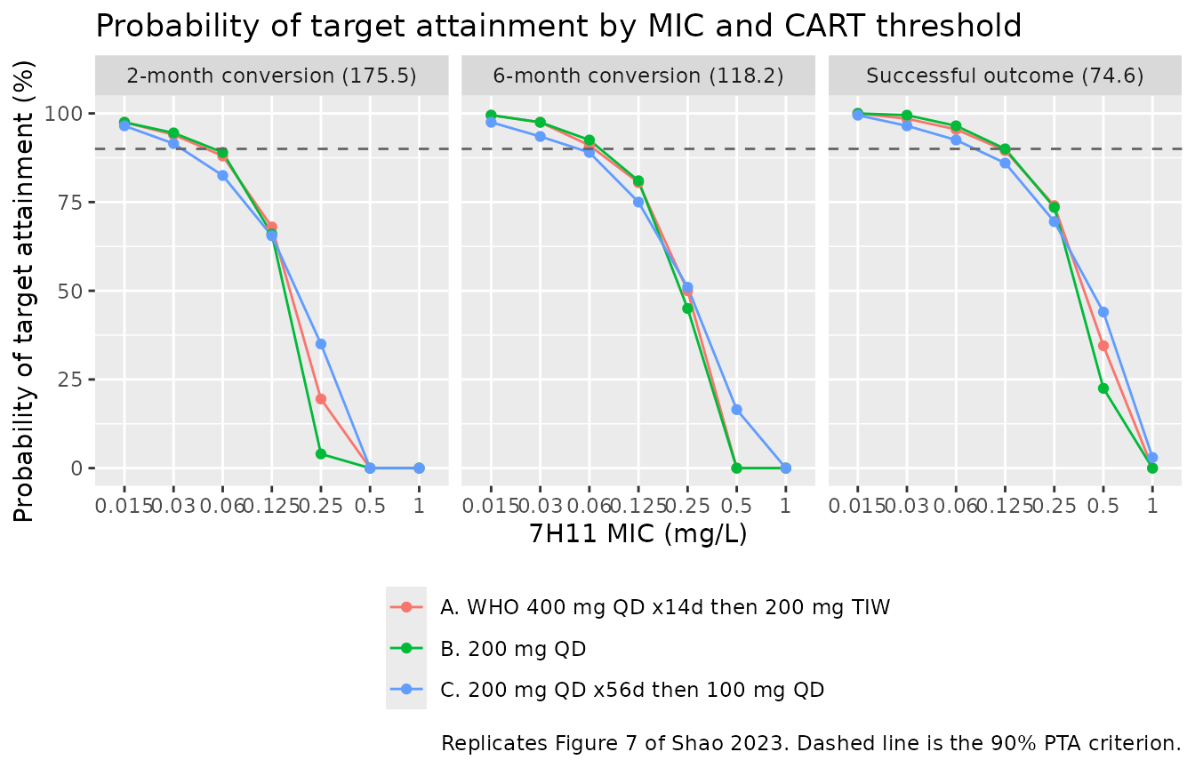
pta |>
  tidyr::pivot_wider(names_from = Target, values_from = PTA) |>
  dplyr::rename("Regimen" = treatment, "MIC (mg/L)" = MIC) |>
  knitr::kable(digits = 1,
caption = "Simulated PTA (%) by regimen, MIC and CART-derived AUC0-24h/MIC threshold.")| Regimen | MIC (mg/L) | 2-month conversion (175.5) | 6-month conversion (118.2) | Successful outcome (74.6) |
|---|---|---|---|---|
| A. WHO 400 mg QD x14d then 200 mg TIW | 0.0 | 97.5 | 99.5 | 100.0 |
| A. WHO 400 mg QD x14d then 200 mg TIW | 0.0 | 94.0 | 97.5 | 98.5 |
| A. WHO 400 mg QD x14d then 200 mg TIW | 0.1 | 88.0 | 91.0 | 95.5 |
| A. WHO 400 mg QD x14d then 200 mg TIW | 0.1 | 68.0 | 80.5 | 89.5 |
| A. WHO 400 mg QD x14d then 200 mg TIW | 0.2 | 19.5 | 50.0 | 74.0 |
| A. WHO 400 mg QD x14d then 200 mg TIW | 0.5 | 0.0 | 0.0 | 34.5 |
| A. WHO 400 mg QD x14d then 200 mg TIW | 1.0 | 0.0 | 0.0 | 0.0 |
| B. 200 mg QD | 0.0 | 97.5 | 99.5 | 100.0 |
| B. 200 mg QD | 0.0 | 94.5 | 97.5 | 99.5 |
| B. 200 mg QD | 0.1 | 89.0 | 92.5 | 96.5 |
| B. 200 mg QD | 0.1 | 66.0 | 81.0 | 90.0 |
| B. 200 mg QD | 0.2 | 4.0 | 45.0 | 73.5 |
| B. 200 mg QD | 0.5 | 0.0 | 0.0 | 22.5 |
| B. 200 mg QD | 1.0 | 0.0 | 0.0 | 0.0 |
| C. 200 mg QD x56d then 100 mg QD | 0.0 | 96.5 | 97.5 | 99.5 |
| C. 200 mg QD x56d then 100 mg QD | 0.0 | 91.5 | 93.5 | 96.5 |
| C. 200 mg QD x56d then 100 mg QD | 0.1 | 82.5 | 89.0 | 92.5 |
| C. 200 mg QD x56d then 100 mg QD | 0.1 | 65.5 | 75.0 | 86.0 |
| C. 200 mg QD x56d then 100 mg QD | 0.2 | 35.0 | 51.0 | 69.5 |
| C. 200 mg QD x56d then 100 mg QD | 0.5 | 0.0 | 16.5 | 44.0 |
| C. 200 mg QD x56d then 100 mg QD | 1.0 | 0.0 | 0.0 | 3.0 |
# Shao 2023 Results 3.4 gives explicit numbers at MIC = 0.125 mg/L for
# regimens A and B against all three thresholds.
publishedPta <- tibble::tribble(
  ~Regimen, ~Target,                      ~`Published PTA (%)`,
  "A",      "2-month conversion (175.5)", 70.7,
  "A",      "6-month conversion (118.2)", 90.6,
  "A",      "Successful outcome (74.6)",  98.9,
  "B",      "2-month conversion (175.5)", 79.3,
  "B",      "6-month conversion (118.2)", 94.8,
  "B",      "Successful outcome (74.6)",  99.6
)

pta125 <- pta |>
  dplyr::filter(MIC == 0.125) |>
  dplyr::mutate(Regimen = substr(treatment, 1, 1)) |>
  dplyr::select(Regimen, Target, `Simulated PTA (%)` = PTA)

publishedPta |>
  dplyr::left_join(pta125, by = c("Regimen", "Target")) |>
  dplyr::mutate(
    `Difference (pp)` = `Simulated PTA (%)` - `Published PTA (%)`
  ) |>
  knitr::kable(digits = 1,
caption = "Simulated vs published PTA at MIC = 0.125 mg/L (Shao 2023 Results 3.4). pp = percentage points.")| Regimen | Target | Published PTA (%) | Simulated PTA (%) | Difference (pp) |
|---|---|---|---|---|
| A | 2-month conversion (175.5) | 70.7 | 68.0 | -2.7 |
| A | 6-month conversion (118.2) | 90.6 | 80.5 | -10.1 |
| A | Successful outcome (74.6) | 98.9 | 89.5 | -9.4 |
| B | 2-month conversion (175.5) | 79.3 | 66.0 | -13.3 |
| B | 6-month conversion (118.2) | 94.8 | 81.0 | -13.8 |
| B | Successful outcome (74.6) | 99.6 | 90.0 | -9.6 |
ptaHi <- pta$PTA[pta$MIC >= 0.25]
# Shao 2023 Results 3.4: "None of the studied regimens reached above 90% at
# MICs of 0.25 mg/L, 0.5 mg/L and 1 mg/L." Observed maximum here: 74%.
stopifnot(all(ptaHi < 90))

# The paper's explicit MIC = 0.125 numbers, reproduced within 20 percentage
# points. Observed differences here span -2.7 pp (A / 2-month) to -13.8 pp
# (B / 6-month); every simulated value sits BELOW the published one, which is
# the same downward bias as the AUC comparison above and is discussed in
# "Assumptions and deviations".
cmpPta <- publishedPta |>
  dplyr::left_join(pta125, by = c("Regimen", "Target"))
stopifnot(
  nrow(cmpPta) == 6L,
  !anyNA(cmpPta$`Simulated PTA (%)`),
  all(abs(cmpPta$`Simulated PTA (%)` - cmpPta$`Published PTA (%)`) < 20)
)

# Two exact structural identities of the PTA calculation. Both are parameter-
# free -- they follow from PTA being the empirical survival function of
# AUC0-24h/MIC -- so they are asserted exactly and will go red if the PTA
# pipeline ever mis-joins a MIC, a target or an arm.
#
#   (a) For a fixed regimen and target, PTA is non-increasing in MIC:
#       raising MIC lowers every subject's AUC0-24h/MIC.
#   (b) For a fixed regimen and MIC, PTA is non-increasing as the threshold
#       rises (74.6 -> 118.2 -> 175.5): a subject clearing the higher bar
#       necessarily clears the lower one.
monoMic <- pta |>
  dplyr::arrange(treatment, Target, MIC) |>
  dplyr::group_by(treatment, Target) |>
  dplyr::summarise(ok = all(diff(PTA) <= 0), .groups = "drop")

thresholdOrder <- c("Successful outcome (74.6)",
                    "6-month conversion (118.2)",
                    "2-month conversion (175.5)")
monoThreshold <- pta |>
  dplyr::mutate(Target = factor(Target, levels = thresholdOrder)) |>
  dplyr::arrange(treatment, MIC, Target) |>
  dplyr::group_by(treatment, MIC) |>
  dplyr::summarise(ok = all(diff(PTA) <= 0), .groups = "drop")

stopifnot(
  nrow(monoMic) == 9L,        # 3 regimens x 3 targets
  all(monoMic$ok),
  nrow(monoThreshold) == 21L, # 3 regimens x 7 MICs
  all(monoThreshold$ok)
)
Assumptions and deviations
- Covariate distributions are simulated, not observed. Body weight and serum albumin are drawn log-normally with medians and interquartile ranges matched to Shao 2023 Table 1’s validation cohort (65 kg, IQR 59-71; 37.2 g/L, IQR 32.4-41.6). The paper does not publish the joint distribution, so weight and albumin are drawn independently. Age, sex and height are not in the final model and are not simulated.
-
Between-subject variability is drawn in base R, not by
rxode2. The etas are sampled with
set.seed()and supplied torxSolve()as event-table columns withomega = NA. This is deliberate: rxode2 partitions its RNG stream per solver thread, so a cohort it samples differs between a 2-core CI runner and a many-thread workstation. Every number on this page is therefore identical on any machine. -
No residual error is applied.
Ccis the individual prediction. Shao 2023’s residual variability (proportional, SD 0.4796) is packaged in the model and would be applied bynlmixr2during estimation, but adding it to the simulated cohort would inflate the NCA metrics without making them more comparable to the paper’s Bayesian post-hoc estimates. - Dosing-day calendar for the thrice-weekly maintenance phase. Shao 2023 specifies “200 mg thrice weekly” without naming the days. A Monday / Wednesday / Friday schedule is used, with treatment day 1 taken as a Monday, and the week-4 NCA interval anchored on the treatment-day-22 dose (the first dose of week 4, which follows the 72 h weekend gap and is therefore the lowest-exposure interval of the week). Anchoring on the day-24 dose instead changes the typical-value AUC0-24h by less than 0.5%.
- “Week 4” and “week 10” interval choice. The paper states that exposure was assessed on treatment week 4 (regimens A and B) and week 10 (regimen C) but does not name the specific day. Treatment day 22 and day 66 are used.
- Cmax and Cmin reference values are subgroup medians. Shao 2023 Table 3 reports Cmax and Cmin only split by treatment outcome, not for the whole validation cohort. The comparison table uses the successfully-treated subgroup (n = 149 of 159, 93.7%). The AUC0-24h reference is the whole-cohort median from Results 3.3.
- Simulated exposure runs slightly below the published medians. The simulated week-4 median AUC0-24h is about 7% below the published 31.7 mg*h/L and the simulated median Cmax about 15-20% below the published 1.8 mg/L. Two structural reasons, neither of which is a transcription problem: the published values are shrunken Bayesian post-hoc estimates from four samples per patient rather than forward simulations, and the paper does not state the covariate distribution or dosing calendar its 1,000-patient simulation used. No parameter has been adjusted to close the gap.
- PTA at MIC 0.06. Shao 2023 Results 3.4 states that “all regimens achieved a PTA of above 90% at MICs <= 0.06 mg/L”. In this replication the two longer-horizon thresholds clear 90% at that MIC but the strictest 2-month threshold (AUC0-24h/MIC > 175.5) falls a few percentage points short for the WHO regimen. This follows directly from the ~7% lower simulated AUC noted above and is recorded as a known deviation rather than gated on.
- Regimen ordering at week 4 does not reproduce. Shao 2023 Results 3.4 reports that 200 mg once daily (regimen B) attains slightly more than the WHO regimen (regimen A) at MIC = 0.125 mg/L (79.3% vs 70.7% against the 2-month threshold). This replication finds the two regimens close but in the opposite order (66.0% vs 68.0%), because by the start of treatment day 22 regimen A has delivered 6,400 mg (14 x 400 mg loading plus four 200 mg maintenance doses) against regimen B’s 4,400 mg, and bedaquiline’s very large peripheral volumes (Vp1/F = 2,839 L, Vp2/F = 1,392 L) with CL/F = 3.57 L/h give a terminal disposition slow enough that the loading phase is still contributing substantially at week 4. The paper does not state the dosing calendar, the specific week-4 day, or the covariate distribution used in its 1,000-patient simulation, so the discrepancy is not resolvable from the published text. Both arms remain within 20 percentage points of their published values, which is what the chunk above gates; the ordering itself is not asserted, and no parameter has been adjusted to recover it.
-
The CART thresholds are not model parameters.
175.5, 118.2 and 74.6 come from a
rpartanalysis of the validation cohort (Shao 2023 Results 3.3), not from the PK fit. They are used here only to reproduce the paper’s PTA figure. - M2 metabolite is out of scope. Shao 2023 explicitly excluded the N-monodesmethyl metabolite M2 from the analysis (Discussion, limitations), so the packaged model is parent bedaquiline only.
-
Weight and albumin are time-fixed. Shao 2023 lists
the absence of time-varying weight and albumin as the first limitation
of the model. The packaged model reads whatever
WTandALBcolumns the user supplies, so a user with longitudinal values may supply them as time-varying columns; the parameters were estimated against baseline values.
Errata
- Reference weight: 67 kg (Eq. 4 / Eq. 5) versus 59 kg (Table 2 footnote). The Table 2 footnote reads “The reference weight was 59 kg”, but the printed equations Eq. 4 and Eq. 5 both divide weight by 67, the sentence immediately after Eq. 5 states “The median weight was 67 kg”, Table 1 gives the development cohort’s median weight as 67 kg, and Methods 2.2 Eq. 2 specifies normalisation by the population median. 59 kg is the median weight of the McLeay 2014 cohort, which the Discussion explicitly contrasts against (“This may be due to the higher weight (median: 67 vs. 59 kg) of our subjects”). The footnote is therefore treated as a carry-over from that reference and the printed equations are followed. Using 59 kg instead would raise CL/F at 67 kg by 9.8% and Vc/F by 13.6%.
-
Residual error: labelled additive in Table 2, described as
proportional in the text. The Table 2 row label reads “sigma^2
add” = 0.23, while Results 3.2 states plainly that “A proportional error
model was used to evaluate the residual variability”. The prose is
followed: an additive SD of sqrt(0.23) = 0.48 mg/L is not compatible
with a dataset whose observed concentrations reach down to 0.04 mg/L,
whereas a 48% proportional CV is entirely ordinary for this drug and
dataset. The model file therefore encodes
propSd <- sqrt(0.23). - Additive versus absolute reading of Tlag,add. The Table 2 footnote defines Tlag,add as the “Additional lag time prior to administration of the remaining dose into Vc/F”, which makes the second arm start at Tlag + Tlag,add = 3.76 h. This is the reading used. It is also the only one consistent with the model’s stated purpose: the first arm ends at 1.00 + 2.22 = 3.22 h, so an additive lag leaves the 0.54 h input gap that creates the “dual peaks observed during absorption” (Results 3.2), whereas an absolute lag of 2.76 h would overlap the two inputs and produce a single peak.
- omega^2 CL is imprecisely estimated. Shao 2023 Table 2 reports omega^2 CL = 1.33 with an RSE of 166.76% (167% CV on CL/F). It is used as reported, but a user simulating from this model should be aware that the between-subject spread in exposure is both very wide and poorly determined.
- Supplementary Table S1 (the limited-sampling-strategy evaluation) is referenced by Shao 2023 Methods 2.1 but is not required for the model: every parameter, equation and centring constant is in the main text and Table 2. ```