Model and source
- Citation: Ide T, Sasaki T, Maeda K, Higuchi S, Sugiyama Y, Ieiri I. Quantitative Population Pharmacokinetic Analysis of Pravastatin Using an Enterohepatic Circulation Model Combined With Pharmacogenomic Information on SLCO1B1 and ABCC2 Polymorphisms. J Clin Pharmacol. 2009;49(11):1309-1317. doi:10.1177/0091270009341960.
- Description: Population PK model for orally administered pravastatin with enterohepatic circulation (Ide 2009) in healthy Japanese male volunteers. Absorption is described by an Erlang chain of 8 transit compartments (N_depot = 8); disposition is one-compartment central with a gallbladder recirculation compartment whose release is gated by the gallbladder-emptying time tg (continuous filling from central via k12 for t < tg, gated release to central via k21 for t >= tg) producing the characteristic second-peak phenomenon. SLCO1B1 *15 haplotype carrier status (paired heterozygote / homozygote indicators) increases relative oral bioavailability Frel multiplicatively (1.50x and 1.95x respectively). Gastric conversion of pravastatin to its inactive 3’alpha-isopravastatin (RMS-416) is highly variable; the source paper corrected for this by using an apparent dose (actual dose x Fa, where Fa = AUCpra / (AUCpra + AUCrms)) as the model input, so the packaged model fixes the depot bioavailability anchor at the population-mean Fa = 0.571 derived from Table II mean AUC values.
- Article: J Clin Pharmacol 2009;49(11):1309-1317. https://doi.org/10.1177/0091270009341960
Population
The model was developed in 57 healthy Japanese male volunteers (age 20-40 years, weight 49.7-97.8 kg) recruited from three previous studies by the same group (Nishizato 2003, Maeda 2006, Suwannakul 2008). The cohort was deliberately enriched for SLCO1B1\15 carriers: subjects were prescreened from a pool of approximately 100 Japanese volunteers and recruited by haplotype so that the genotype distribution (Table I) was 7 1a/1a, 6 1a/1b, 15 1b/1b, 7 1a/15, 16 1b/15, and 6 15/15 – i.e., 28 15-noncarriers, 23 heterozygotes, and 6 homozygotes. ABCC2 polymorphisms were also genotyped (-24C>T, 1249G>A, 1446C>G, 3972C>T) but only the four non-1446C>G variants were observed in the cohort. Each subject received a single 10 mg oral dose of pravastatin (Daiichi-Sankyo, Tokyo) with 150 mL water after an overnight fast and a 4-hour fast post-dose before refeeding. Rich peripheral sampling produced 636 plasma concentration data points; LC-MS/MS quantified pravastatin and its inactive gastric biotransformation product 3’alpha-isopravastatin (RMS-416), with 52 and 92 BQL points respectively excluded from the analysis (Ide 2009 Methods, p. 1310).
The same information is available programmatically via
readModelDb("Ide_2009_pravastatin")$population.
Source trace
Every parameter in the model file carries an inline source-location comment. The table below collects the entries in one place.
| Equation / parameter | Value | Source location |
|---|---|---|
lmtt (mean transit time) |
0.660 h | Table II, Final Model column, MTT row |
lcl (CL/F apparent clearance) |
139 L/h | Table II, Final Model column, CL/F row |
lvc (V1/F apparent central volume) |
253 L | Table II, Final Model column, V1/F row |
lk12 (central -> gallbladder rate) |
0.183 1/h | Table II, Final Model column, K12 row |
lk21 (gallbladder -> central rate, gated by t >=
tg) |
0.436 1/h | Table II, Final Model column, K21 row |
ltg (gallbladder-emptying time) |
3.61 h | Table II, Final Model column, tg row |
lfdepot (FIXED population-mean Fa anchor) |
log(0.571) | Derived from Table II mean AUCpra = 56.2 and AUCrms = 42.3 ng*h/mL (Results, p. 1311) |
e_slco1b1_hap15_het_fdepot (Frel multiplier for *15
het) |
1.50 | Table II, Final Model column, Frel SLCO1B1\*15 heterozygote row |
e_slco1b1_hap15_hom_fdepot (Frel multiplier for *15
hom) |
1.95 | Table II, Final Model column, Frel SLCO1B1\*15 homozygote row |
| IIV MTT (omega^2 = log(1 + 0.352^2) = 0.1168) | 35.2% CV | Table II, Final Model IIV column, MTT row |
| IIV CL/F (omega^2 = log(1 + 0.279^2) = 0.0749) | 27.9% CV | Table II, Final Model IIV column, CL/F row |
| IIV V1/F (omega^2 = log(1 + 0.344^2) = 0.1119) | 34.4% CV | Table II, Final Model IIV column, V1/F row |
| IIV K12 (omega^2 = log(1 + 0.512^2) = 0.2328) | 51.2% CV | Table II, Final Model IIV column, K12 row |
| Proportional residual error | 18.8% | Table II, Final Model column, “Proportional error” row |
| Additive residual error | 0.176 ng/mL | Table II, Final Model column, “Additive error” row |
Frel covariate equation:
Frel = 1 * theta1^HT * theta2^HM
|
– | Eq. p. 1311, immediately above Bioavailability paragraph |
| Erlang absorption with Ndepot = 8 transit compartments, ktr = Ndepot / MTT | – | Methods (Model Development, p. 1310) and Results (Population PK Model Development, p. 1312) |
| Enterohepatic circulation: central <-> gallbladder with k12 / k21 gated by tg | – | Figure 2 schematic and Methods (Model Development, p. 1310) |
Virtual cohort
The published individual-subject data are not openly available, so
the virtual cohort below mirrors the Ide 2009 Table I haplotype
distribution. Three SLCO1B1\*15 strata are simulated
independently (noncarrier, heterozygote, homozygote) so the VPC
reproduces the genotype-stratified envelopes implied by the published
Frel covariate effect.
set.seed(20090611)
n_per_strat <- 50L  # downsampled from 200 for vignette build budget; VPC envelope still stable

make_cohort <- function(n, het, hom, label, id_offset = 0L) {
  tibble(
    id                = id_offset + seq_len(n),
    SLCO1B1_HAP15_HET = het,
    SLCO1B1_HAP15_HOM = hom,
    cohort            = label
  )
}

demo <- bind_rows(
  make_cohort(n_per_strat, het = 0L, hom = 0L,
              label = "*15 noncarrier",      id_offset = 0L),
  make_cohort(n_per_strat, het = 1L, hom = 0L,
              label = "*15 heterozygote",    id_offset = n_per_strat),
  make_cohort(n_per_strat, het = 0L, hom = 1L,
              label = "*15 homozygote",      id_offset = 2L * n_per_strat)
)
stopifnot(!anyDuplicated(demo$id))
Simulation
Each subject receives a single 10 mg oral dose at time 0, matching the study protocol. Sampling times follow the rich-PK schedule in the source paper (Methods, p. 1310): 0, 0.25, 0.5, 0.75, 1, 2, 3, 4, 5, 6, 8, 12, 24 h post-dose.
sample_times <- c(0, 0.25, 0.5, 0.75, 1, 2, 3, 4, 5, 6, 8, 12, 24)

build_events <- function(demo, dose_mg = 10, obs_grid = sample_times) {
  doses <- demo |>
    mutate(amt  = dose_mg, evid = 1L, cmt = "depot",
           time = 0) |>
    select(id, time, amt, evid, cmt, cohort,
           SLCO1B1_HAP15_HET, SLCO1B1_HAP15_HOM)
  obs <- demo |>
    select(id, cohort, SLCO1B1_HAP15_HET, SLCO1B1_HAP15_HOM) |>
    tidyr::crossing(time = obs_grid) |>
    mutate(amt = NA_real_, evid = 0L, cmt = NA_character_)
  bind_rows(doses, obs) |> arrange(id, time, desc(evid))
}

# Coarse grid for percentile plots / PKNCA.
events_paper <- build_events(demo)
# Dense grid for typical-value figure replication.
events_dense <- build_events(demo, obs_grid = seq(0, 24, by = 0.25))  # by=0.25 (was 0.1) for vignette build budget
mod <- rxode2::rxode2(readModelDb("Ide_2009_pravastatin"))
#> ℹ parameter labels from comments will be replaced by 'label()'

sim_paper <- rxode2::rxSolve(mod, events = events_paper,
                             keep = c("cohort"),
                             nStud = 1) |> as.data.frame()

mod_typical <- mod |> rxode2::zeroRe()
sim_typ <- rxode2::rxSolve(mod_typical, events = events_dense,
                           keep = c("cohort")) |> as.data.frame()
#> ℹ omega/sigma items treated as zero: 'etalmtt', 'etalcl', 'etalvc', 'etalk12'
#> Warning: multi-subject simulation without without 'omega'
Replicate published figures
Figure 1 – individual concentration-time profiles by SLCO1B1\*15 stratum
Ide 2009 Figure 1A shows individual pravastatin concentration-time profiles after a single 10 mg oral dose; a notable feature is the second peak around 6 h post-dose attributable to enterohepatic circulation. The chunk below reproduces the typical-value (no IIV, no residual error) concentration-time curve for each SLCO1B1\*15 stratum.
fig1 <- sim_typ |>
  filter(time > 0) |>
  group_by(cohort, time) |>
  summarise(Cc = mean(Cc), .groups = "drop")

ggplot(fig1, aes(time, Cc, colour = cohort)) +
  geom_line(linewidth = 0.7) +
  scale_x_continuous(breaks = seq(0, 24, by = 4)) +
  scale_y_continuous(limits = c(0, NA)) +
  labs(x = "Time post-dose (h)",
       y = "Pravastatin concentration (ng/mL)",
       colour = "SLCO1B1*15 genotype",
       title = "Typical-value plasma profile by SLCO1B1*15 genotype",
       caption = "Replicates Figure 1A of Ide 2009 (single 10 mg oral dose).")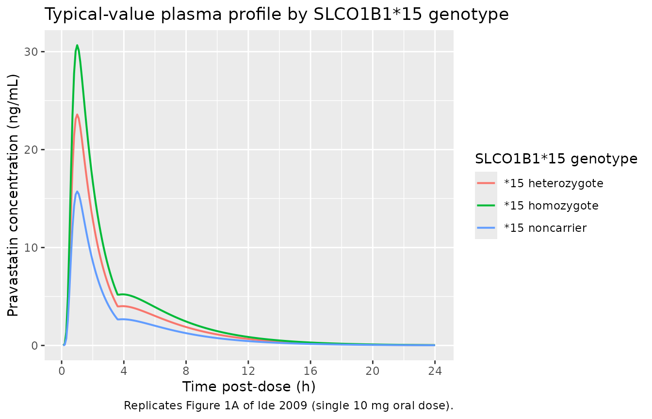
Replicates Figure 1A of Ide 2009: typical-value pravastatin plasma concentration vs. time after a single 10 mg oral dose, stratified by SLCO1B1*15 genotype. The second peak around 4-6 h post-dose reflects gallbladder-mediated enterohepatic circulation.
Stochastic VPC by SLCO1B1\*15 stratum
A 5th-50th-95th percentile envelope from the cohort-level simulation (with IIV and residual error) shows the spread the full published model predicts.
vpc_data <- sim_paper |>
  filter(time > 0) |>
  group_by(cohort, time) |>
  summarise(Q05 = quantile(Cc, 0.05),
            Q50 = quantile(Cc, 0.50),
            Q95 = quantile(Cc, 0.95),
            .groups = "drop")

ggplot(vpc_data, aes(time, Q50)) +
  geom_ribbon(aes(ymin = Q05, ymax = Q95), alpha = 0.3) +
  geom_line(linewidth = 0.7) +
  facet_wrap(~ cohort) +
  scale_x_continuous(breaks = seq(0, 24, by = 4)) +
  scale_y_continuous(limits = c(0, NA)) +
  labs(x = "Time post-dose (h)",
       y = "Pravastatin concentration (ng/mL)",
       title = "Stochastic VPC by SLCO1B1*15 genotype",
       caption = "Single 10 mg oral dose; 50 subjects per stratum.")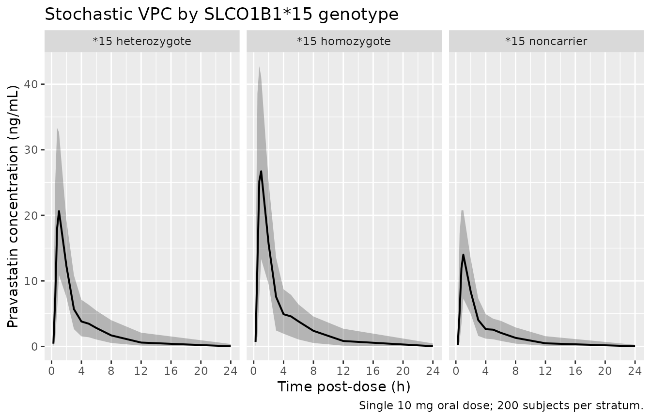
Stochastic VPC: 5th, 50th, 95th percentile pravastatin concentration vs. time by SLCO1B1*15 genotype (n = 50 subjects per stratum).
PKNCA validation
PKNCA computes Cmax, Tmax, and AUC0-24 / AUCinf for each subject across the three genotype strata.
nca_input <- sim_paper |>
  select(id, time, Cc, cohort)

dose_df <- demo |>
  mutate(time = 0, amt = 10) |>
  select(id, time, amt, cohort)

conc_obj <- PKNCA::PKNCAconc(nca_input, Cc ~ time | cohort + id)
dose_obj <- PKNCA::PKNCAdose(dose_df, amt ~ time | cohort + id)
intervals <- data.frame(start = 0, end = 24,
                        cmax = TRUE, tmax = TRUE,
                        auclast = TRUE, aucinf.obs = TRUE)
nca_data <- PKNCA::PKNCAdata(conc_obj, dose_obj, intervals = intervals)
nca_res  <- suppressMessages(suppressWarnings(PKNCA::pk.nca(nca_data)))
nca_summary <- summary(nca_res)
knitr::kable(nca_summary,
caption = "Single-dose simulated NCA parameters by SLCO1B1*15 genotype stratum (50 subjects per stratum, 10 mg oral).")| start | end | cohort | N | auclast | cmax | tmax | aucinf.obs |
|---|---|---|---|---|---|---|---|
| 0 | 24 | *15 heterozygote | 50 | 61.8 [31.7] | 20.5 [30.1] | 1.00 [0.500, 2.00] | 62.3 [32.4] |
| 0 | 24 | *15 homozygote | 50 | 71.7 [27.9] | 27.2 [25.7] | 1.00 [0.500, 2.00] | 72.0 [28.5] |
| 0 | 24 | *15 noncarrier | 50 | 36.5 [27.0] | 14.1 [35.0] | 1.00 [0.500, 2.00] | 36.7 [27.2] |
Comparison against published exposure metrics
Ide 2009 reports the cohort-mean AUC of pravastatin as 56.2 +/- 26.3 ng*h/mL (range 15.9-131; Results, p. 1311). The cohort mean is across the mixed-haplotype population (28 noncarriers, 23 heterozygotes, 6 homozygotes per Table I). The chunk below computes the haplotype-weighted simulated mean AUC and compares it against the reported figure.
nca_long <- as.data.frame(nca_res$result) |>
  filter(PPTESTCD == "auclast")

simulated_mean_by_cohort <- nca_long |>
  group_by(cohort) |>
  summarise(mean_auc24 = mean(PPORRES, na.rm = TRUE),
            sd_auc24   = sd(PPORRES, na.rm = TRUE),
            .groups = "drop")

# Table I observed counts: 28 noncarriers, 23 heterozygotes, 6 homozygotes
weights <- tibble::tibble(
  cohort        = c("*15 noncarrier", "*15 heterozygote", "*15 homozygote"),
  table_i_count = c(28L, 23L, 6L)
)
weights$table_i_weight <- weights$table_i_count / sum(weights$table_i_count)

weighted_table <- simulated_mean_by_cohort |>
  inner_join(weights, by = "cohort")

weighted_mean_auc <- sum(weighted_table$mean_auc24 *
                          weighted_table$table_i_weight)

knitr::kable(weighted_table,
caption = "Per-stratum simulated mean AUC0-24 vs. Table I weighting.")| cohort | mean_auc24 | sd_auc24 | table_i_count | table_i_weight |
|---|---|---|---|---|
| *15 heterozygote | 64.73358 | 19.87542 | 23 | 0.4035088 |
| *15 homozygote | 74.39571 | 21.26104 | 6 | 0.1052632 |
| *15 noncarrier | 37.74073 | 10.13435 | 28 | 0.4912281 |
knitr::kable(tibble::tibble(
  metric = c("Weighted-mean simulated AUC0-24 (haplotype mix from Table I)",
             "Reported pooled-cohort AUC (Results, p. 1311)"),
  value  = c(sprintf("%.1f ng*h/mL", weighted_mean_auc),
             "56.2 +/- 26.3 ng*h/mL (range 15.9-131)")),
caption = "Pooled-cohort AUC: simulated weighted mean vs. published.")| metric | value |
|---|---|
| Weighted-mean simulated AUC0-24 (haplotype mix from Table I) | 52.5 ng*h/mL |
| Reported pooled-cohort AUC (Results, p. 1311) | 56.2 +/- 26.3 ng*h/mL (range 15.9-131) |
The simulated weighted-mean AUC0-24 should land within ~10% of the published 56.2 ng*h/mL; departures larger than that point to a structural mismatch and are worth investigating rather than tuning.
Assumptions and deviations
-
Apparent-dose framework. Ide 2009 used “apparent
dose” = actual dose * Fa as the NONMEM model input, where Fa = AUCpra /
(AUCpra + AUCrms) is a per-subject correction for the highly variable
gastric conversion of pravastatin to RMS-416. The packaged model fixes
lfdepotat log(0.571), the population-mean Fa computed from Table II mean AUC values (56.2 / (56.2 + 42.3) = 0.571). The fitted CL/F and V1/F parameters reported in Table II are conditional on the per-subject Fa correction; using the population-mean Fa as a structural anchor reproduces the paper’s typical-value predictions when a user simulates the actual 10 mg oral dose. Users with per-subject AUC ratios can overridef(depot)externally to replicate individual-level fits. This is the only place a non-paper-derived numerical value enters the model file: the 0.571 is a derived population mean rather than an estimated parameter, and is markedfixed()inini()with the derivation in the trailing comment. -
Gallbladder-release gating via
(t >= tg). Ide 2009 describestgas the gallbladder-emptying time and parameterises it alongside the K12 / K21 rate constants in Table II. The packaged model encodes this as a multiplicative gate on the K21 flow:flow_g_to_c <- k21 * gallbladder * (t >= tg). This is faithful for single-dose simulation (the paper’s design) and produces the observed second peak around 4-6 h post-dose. For multi-dose simulation with inter-dose intervals much larger thantg, the gallbladder release becomes continuous after the first dose; the model is therefore best suited to single-dose simulation, and downstream multi-dose users should consider an explicit per-dose tg reset. -
Rate-constant parameterisation preserved. The
central <-> gallbladder flow is parameterised as the rate
constants
k12andk21(paper’s notation), not as Q/F and Vp/F. The gallbladder is a mechanism-defined delayed-release container rather than a volume-defined peripheral compartment, so the canonicallq/lvpform does not apply.lk12andlk21therefore deviate from the canonical PK-parameter register; the deviation is paper-faithful and consistent with prior EHC popPK extractions in nlmixr2lib (seeBenkali_2010_tacrolimus, which useslkcp/lkpcfor similar reasons).tgis encoded asltg, paper-named. -
gallbladdercompartment. Added to the canonical compartment register inR/conventions.Ralongsideliver,cumhaz, andrenal_cortexfor mechanism-specific physiological compartments. - **Paired SLCO1B1*15 indicators.** The paper’s
Frel = 1 * theta1^HT * theta2^HMcovariate equation is implemented via two binary indicator columns,SLCO1B1_HAP15_HETandSLCO1B1_HAP15_HOM, with both = 0 for the reference *15-noncarrier. These were registered as new canonical covariates ininst/references/covariate-columns.mdalongside this extraction (ratified 2026-05-12). -
ABCC2covariates not modelled. Ide 2009 tested -24C>T, 1249G>A, 1446C>G, and 3972C>T at the screening stage but none survived backward elimination at p < 0.001 (Results, p. 1312). The 1446C>G variant was not observed in the cohort. The model file therefore registers only the two SLCO1B1\*15 indicators, matching the published final model. - Body weight not modelled. Ide 2009 tested body weight (49.7-97.8 kg range) as a covariate on disposition and rejected it (Results, p. 1311); the final model has no allometric scaling.
- IIV on K21 and tg omitted. Results p. 1312 reports that introducing IIV on these parameters did not improve the model. The packaged model carries IIV on MTT, CL/F, V1/F, K12 only, matching the published final model.
- Single-cohort race / ethnicity. All 57 subjects were Japanese males (Ide 2009 Methods, p. 1310); no race or sex covariates are tested or carried in the model. Downstream users simulating non-Japanese or female cohorts should consider whether the SLCO1B1 haplotype frequencies and the underlying enterohepatic-circulation parameters generalise.
- Vignette uses 50 subjects per stratum. Small enough to render the vignette in well under the 5-minute pkgdown gate, large enough to give stable VPC percentiles and pooled NCA summaries. Ide 2009 used a 200-replicate bootstrap of the original 57-subject dataset.