Model and source
- Citation: Chung TK, Lee HA, Park SI, Oh DY, Lee KW, Kim JW, Kim JH, Woo A, Lee SJ, Bang YJ, Lee H (2021). A target-mediated drug disposition population pharmacokinetic model of GC1118, a novel anti-EGFR antibody, in patients with solid tumors. Clinical and Translational Science 14(3):990-1001. doi:10.1111/cts.12963. Model code from the Supporting Information (NONMEM control stream CTS-14-990-s001.docx).
- Description: Two-compartment target-mediated drug disposition (TMDD) population PK model for GC1118, a fully human anti-EGFR IgG1 monoclonal antibody, in adults with advanced solid tumours (Chung 2021; phase I, n = 32, 2-h IV infusions of 0.3-5 mg/kg once weekly or 8 mg/kg every two weeks). EGFR is confined to the peripheral compartment; drug-EGFR binding is at rapid equilibrium (quasi-equilibrium closed form for the complex), the total peripheral EGFR pool is constant at VP * RB / CLB, and the EGFR and complex clearances are assumed equal. Linear clearance of free drug scales with (WT/70)^0.8. The infusion duration is estimated (D1), a full 9 x 9 IIV block includes IIV on the residual-error magnitude, and inter-occasion variability (two occasions) sits on Q. The peripheral EGFR occupancy (RO, %) is returned as a derived output.
- Article: https://doi.org/10.1111/cts.12963 (open access)
- Supplement: NONMEM control stream (Supporting Information
CTS-14-990-s001.docx), available from the article page and from Europe PMC (PMC8212746).
GC1118 is a fully human IgG1 monoclonal antibody against the epidermal growth factor receptor (EGFR). Chung 2021 fitted a two-compartment target-mediated drug disposition (TMDD) model to the phase I serum concentrations and used it to simulate EGFR occupancy (RO) for once-weekly (Q1W) and every-two-weeks (Q2W) regimens.
Population
The phase I trial enrolled 32 Korean adults with advanced solid tumours (Chung 2021 Table 1): 20 men and 12 women, age 56.7 +/- 9.1 years (range 34-72), body weight 63.1 +/- 10.4 kg (range 42.5-89.2). Colorectal cancer was the primary tumour in 18 patients (56.2%); the remainder had ampulla of Vater, appendix, breast, biliary, oesophageal, gallbladder, gastric, nasal cavity, nasopharyngeal, pancreatic or tonsil cancer. Cohorts 1-5 (n = 24) received a 2-h IV infusion of 0.3, 1, 3, 5 or 4 mg/kg on days 1, 8, 15 and 22; cohort 6 (n = 8) received 8 mg/kg every two weeks. The analysis used 793 free serum GC1118 concentrations (ELISA, LLOQ 0.025 ug/mL). All patients had normal renal and hepatic function and none developed anti-drug antibodies.
The same information is available programmatically via
readModelDb("Chung_2021_GC1118")()$population.
Model structure
EGFR is assumed to be confined to the peripheral compartment, where
drug and receptor bind at rapid equilibrium. The states are the free
drug amount in the central compartment, central
(),
and the total (free + EGFR-bound) drug amount in the
peripheral compartment, peripheral1
(),
both in pmol:
with and the quasi-equilibrium complex
The total peripheral EGFR pool
is constant because the EGFR and complex clearances are assumed equal
().
Receptor occupancy is
.
Doses in mg are converted to pmol with the control stream’s molecular
weight (150 kDa, MWT = 0.15 ug/pmol), and the observed free
serum concentration is
in ug/mL.
Source trace
| Equation / parameter | Value | Source location |
|---|---|---|
d/dt(central) |
n/a | Eq. 1; control stream DADT(1)
|
d/dt(peripheral1) |
n/a | Eq. 2; control stream DADT(2)
|
free_p, complex
|
n/a | Eqs. 3-4; control stream FAP, CPLXP
|
rtot |
vp * ksyn / cl_complex |
Eq. 5; control stream TBP
|
RO |
100 * complex / rtot |
Eq. 9; control stream SAT
|
mw, f(central)
|
0.15 ug/pmol; 1000 / mw
|
control stream MWT = 0.15, F1 = 1/MWT
(stream doses in ug; the library doses in mg) |
dur(central) |
d1 |
control stream D1; Table 2 |
lcl (CLA) |
16.2 mL/h | Table 2 |
e_wt_cl |
0.8, reference 70 kg | Table 2; Methods Eq. 8; control stream
(WT/70)**THETA(11)
|
lvc (VC) |
3660 mL | Table 2 |
lq (Q) |
627 mL/h | Table 2 |
lvp (VP) |
1180 mL | Table 2 |
ld1 (D1) |
2.2 h | Table 2 |
lksyn (RB) |
2390 pmol/h | Table 2 |
lcl_complex (CLB = CLC) |
63.4 mL/h | Table 2 |
lkd (KD) |
0.16 nM, fixed | Table 2; Methods (in vitro value) |
| IIV variances (9) | CV% 36.2, 21.4, 181.4, 58, 6.0, 49.7, 188.1, 227.8, 31.4 | Table 2 IIV column; omega^2 = (CV/100)^2 (see
below) |
| IIV covariances | Table 2 correlation matrix | Table 2 lower panel; order matches control stream
$OMEGA BLOCK(9)
|
etaiov_q_1, etaiov_q_2
|
261.5% CV, shared | Table 2 IOV column; control stream $OMEGA BLOCK(1) +
BLOCK(1) SAME
|
propSd |
0.10 | Table 2 ‘Proportional RUV’ |
addSd |
0.001 ug/mL, fixed | control stream $THETA (0.001) FIX ; Additive error
|
etapropSd |
31.4% CV | Table 2 RUV IIV; control stream
Y = IPRED + W*EPS(1)*EXP(ETA(9))
|
Reconstructing the IIV matrix
Table 2 reports each IIV as a CV% and prints the correlation matrix between the nine IIV terms to three decimals. That printed matrix is very slightly indefinite, which is what rounding a near-singular 9 x 9 correlation matrix (and taking bootstrap medians element by element, as the table heading suggests) can produce. The model uses the nearest positive-definite correlation matrix; the check below shows that no coefficient moved by more than 0.00075, i.e. by about the size of the rounding in the printed table.
cv <- c(CLA = 36.2, VC = 21.4, Q = 181.4, VP = 58, D1 = 6.0, RB = 49.7,
        CLB = 188.1, KD = 227.8, RUV = 31.4) / 100
lower <- list(
  c(1),
  c(0.022, 1),
  c(-0.116, -0.281, 1),
  c(-0.667, 0.272, -0.424, 1),
  c(0.737, 0.218, -0.249, -0.267, 1),
  c(-0.662, 0.649, -0.017, 0.729, -0.268, 1),
  c(-0.311, 0.579, -0.085, 0.642, -0.131, 0.805, 1),
  c(-0.549, 0.333, 0.346, 0.583, -0.364, 0.805, 0.847, 1),
  c(-0.052, -0.317, 0.790, -0.148, 0.027, -0.033, -0.016, 0.414, 1)
)
r_printed <- matrix(0, 9, 9, dimnames = list(names(cv), names(cv)))
for (i in 1:9) r_printed[i, 1:i] <- lower[[i]]
r_printed[upper.tri(r_printed)] <- t(r_printed)[upper.tri(r_printed)]

mod <- readModelDb("Chung_2021_GC1118")
ui <- rxode2::rxode(mod)
#> ℹ parameter labels from comments will be replaced by 'label()'
#> Warning: some etas defaulted to non-mu referenced, possible parsing error: etaiov_q_1, etaiov_q_2
#> as a work-around try putting the mu-referenced expression on a simple line
om <- ui$omega
eta_names <- c("etalcl", "etalvc", "etalq", "etalvp", "etald1", "etalksyn",
               "etalcl_complex", "etalkd", "etapropSd")
om9 <- om[eta_names, eta_names]
r_model <- stats::cov2cor(om9)

data.frame(
  quantity = c("smallest eigenvalue, printed correlation matrix",
               "smallest eigenvalue, model correlation matrix",
               "largest |model - printed| correlation",
               "largest |model SD - Table 2 CV/100|"),
  value = c(min(eigen(r_printed)$values), min(eigen(r_model)$values),
            max(abs(r_model - r_printed)), max(abs(sqrt(diag(om9)) - cv)))
) |>
knitr::kable(digits = 6)| quantity | value |
|---|---|
| smallest eigenvalue, printed correlation matrix | -0.001354 |
| smallest eigenvalue, model correlation matrix | 0.000407 |
| largest |model - printed| correlation | 0.000755 |
| largest |model SD - Table 2 CV/100| | 0.000001 |
stopifnot(
  min(eigen(r_printed)$values) < 0,
  min(eigen(r_model)$values) > 0,
  max(abs(r_model - r_printed)) < 0.001,
  max(abs(sqrt(diag(om9)) - cv)) < 1e-5
)
Which CV% convention?
Chung 2021 does not say how CV% was computed from the variance. With
CVs up to 261.5% the two usual readings differ about three-fold:
omega^2 = (CV/100)^2 (the square-root approximation that
NONMEM/PsN reports print) or omega^2 = log((CV/100)^2 + 1)
(the exact log-normal CV). The paper’s own simulation settles it. Figure
5 shows the mean EGFR occupancy at trough dipping to about 82% after a
first 3 mg/kg dose, and a 5th percentile at steady-state trough of 16.1%
for 8 mg/kg Q2W. Only the square-root reading leaves enough spread in Q,
CLB and RB to produce that; with the log-normal reading, mean trough RO
stays above 95% for every regimen (the comparison below runs both). The
model therefore uses omega^2 = (CV/100)^2. That is also the
reading closer to the initial $OMEGA estimates printed in
the control stream (for example 2.87 and 3.58 on CLB and KD, against
3.54 and 5.19 for the square-root reading and 1.51 and 1.82 for the
log-normal one).
Virtual cohort and simulation of Figure 5
Chung 2021 simulated 3, 4 and 5 mg/kg Q1W and 8 and 10 mg/kg Q2W (2-h
infusions), with body weight distributed as in the analysis dataset. The
virtual cohort draws weight from a normal distribution with the Table 1
mean and SD, redrawing values outside the observed 42.5-89.2 kg range,
and simulates 200 subjects per regimen for 12 weeks. Figure 5 plots the
first dosing interval (days 0-14) and the steady-state window (days
70-84). The two IOV occasions are assigned to those two windows:
OCC = 1 until the day-70 dose and OCC = 2 from
then on.
rxode2::rxSetSeed(20210301)
set.seed(20210301)
n_per_arm <- 200

draw_wt <- function(n) {
  wt <- numeric(0)
  while (length(wt) < n) {
    x <- rnorm(n, 63.1, 10.4)
    wt <- c(wt, x[x >= 42.5 & x <= 89.2])
  }
  wt[seq_len(n)]
}

regimens <- tibble::tribble(
  ~regimen,          ~dose_mgkg, ~tau_h,
  "3 mg/kg Q1W",      3,          168,
  "4 mg/kg Q1W",      4,          168,
  "5 mg/kg Q1W",      5,          168,
  "8 mg/kg Q2W",      8,          336,
  "10 mg/kg Q2W",    10,          336
)

obs_times <- sort(unique(c(
  seq(0, 14 * 24, by = 6), seq(70 * 24, 84 * 24, by = 6),
  7 * 24 - 0.01, 14 * 24 - 0.01, 77 * 24 - 0.01, 84 * 24 - 0.01
)))

make_regimen <- function(k, id_offset) {
  reg <- regimens[k, ]
  ids <- id_offset + seq_len(n_per_arm)
  subj <- tibble(id = ids, WT = draw_wt(n_per_arm))
  dose_times <- seq(0, 12 * 168 - 1, by = reg$tau_h)
  doses <- tidyr::expand_grid(id = ids, time = dose_times) |>
    mutate(evid = 1L, cmt = "central", rate = -2)
  obs <- tidyr::expand_grid(id = ids, time = obs_times) |>
    mutate(evid = 0L, cmt = "central", rate = 0)
  bind_rows(doses, obs) |>
    left_join(subj, by = "id") |>
    mutate(
      amt = ifelse(evid == 1L, reg$dose_mgkg * WT, 0),
      OCC = ifelse(time < 70 * 24, 1L, 2L),
      regimen = reg$regimen
    ) |>
    arrange(id, time, desc(evid))
}

events <- bind_rows(lapply(seq_len(nrow(regimens)), function(k) {
  make_regimen(k, id_offset = (k - 1L) * n_per_arm)
}))
stopifnot(!anyDuplicated(unique(events[, c("id", "time", "evid")])))
The IIV and IOV on Q together have a standard deviation of about 3.2 on the log scale, so an occasional simulated subject has an extreme Q (105-106 mL/h) that makes the system stiff. The solver’s step limit is raised so every subject integrates, and the simulation is checked for missing values.
sim <- rxode2::rxSolve(mod, events = events, keep = c("regimen", "WT"),
                       maxsteps = 1e6, returnType = "data.frame")
#> ℹ parameter labels from comments will be replaced by 'label()'
#> Warning: some etas defaulted to non-mu referenced, possible parsing error: etaiov_q_1, etaiov_q_2
#> as a work-around try putting the mu-referenced expression on a simple line
stopifnot(!anyNA(sim$Cc), !anyNA(sim$RO))
sim$regimen <- factor(sim$regimen, levels = regimens$regimen)
sim_win <- sim |>
  filter(time <= 14 * 24 | time >= 70 * 24) |>
  mutate(window = ifelse(time <= 14 * 24, "After first dose (days 0-14)",
                         "Steady state (days 70-84)"),
         day = time / 24)

fig5_conc <- sim_win |>
  group_by(regimen, window, day) |>
  summarise(mean_Cc = mean(Cc), .groups = "drop")
fig5_ro <- sim_win |>
  group_by(regimen, window, day) |>
  summarise(mean_RO = mean(RO), p05 = quantile(RO, 0.05),
            p95 = quantile(RO, 0.95), .groups = "drop")

ggplot(filter(fig5_conc, mean_Cc > 0), aes(day, mean_Cc, colour = regimen)) +
  geom_line() +
  facet_wrap(~window, scales = "free_x") +
  scale_y_log10() +
  labs(x = "Time (day)", y = "Mean GC1118 concentration (ug/mL)",
       colour = NULL,
       title = "Figure 5a-b: mean simulated concentrations",
       caption = "Replicates Figure 5a-b of Chung 2021.")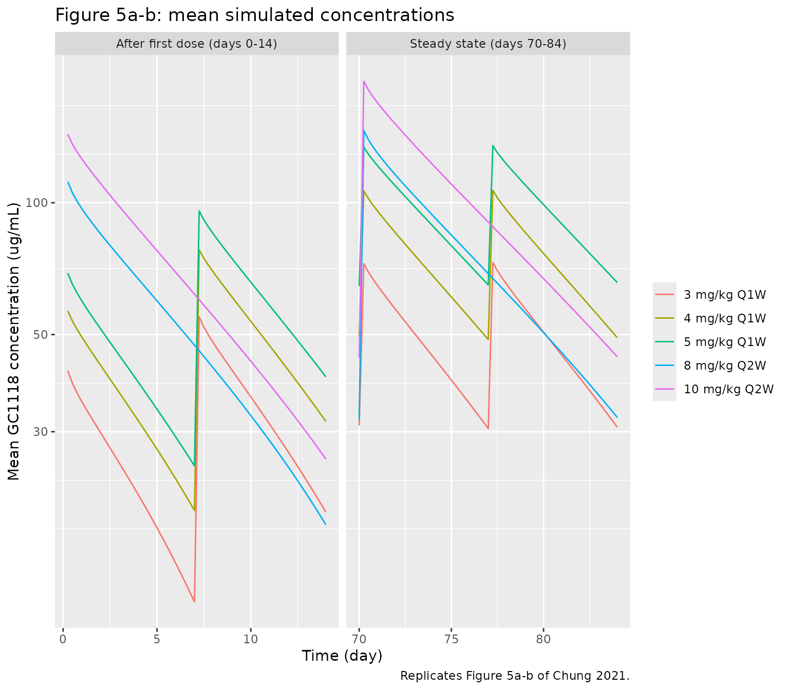
ggplot(fig5_ro, aes(day, mean_RO, colour = regimen)) +
  geom_line() +
  geom_line(aes(y = p05), linetype = "dashed") +
  facet_wrap(~window, scales = "free_x") +
  coord_cartesian(ylim = c(0, 100)) +
  labs(x = "Time (day)", y = "EGFR occupancy (%)", colour = NULL,
       title = "Figure 5c-d: mean (solid) and 5th percentile (dashed) RO",
       caption = "Replicates Figure 5c-d of Chung 2021.")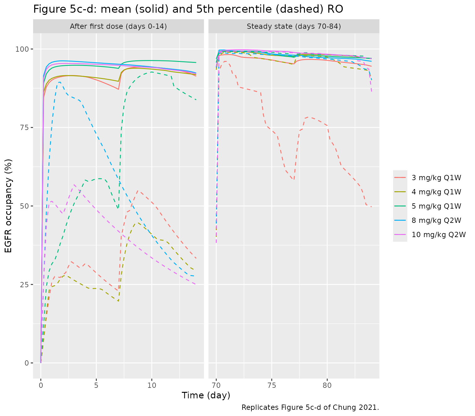
Comparison with the published occupancy and trough values
The published values are the Results text (steady-state trough RO 5th percentiles 87.1%, 99.5%, 16.1% and 41.1% for 4 and 5 mg/kg Q1W and 8 and 10 mg/kg Q2W; mean steady-state trough concentrations 48.57 ug/mL for 4 mg/kg Q1W and 35.67 ug/mL for 8 mg/kg Q2W, Discussion) and, for the mean RO and the 3 mg/kg Q1W percentile, values read by the maintainers from Figure 5c-d.
trough_times <- c(7 * 24, 14 * 24, 77 * 24, 84 * 24) - 0.01
troughs <- sim |>
  filter(time %in% trough_times) |>
  mutate(
    interval = ifelse(time < 70 * 24, "first", "steady state"),
    is_trough = (grepl("Q1W", regimen) & time %in% (c(7, 77) * 24 - 0.01)) |
      (grepl("Q2W", regimen) & time %in% (c(14, 84) * 24 - 0.01))
  ) |>
  filter(is_trough)

sim_summary <- troughs |>
  group_by(regimen, interval) |>
  summarise(mean_RO = mean(RO), p05_RO = quantile(RO, 0.05),
            mean_Cc = mean(Cc), .groups = "drop")

published <- tibble::tribble(
  ~regimen,        ~interval,       ~pub_mean_RO, ~pub_p05_RO, ~pub_mean_Cc,
  "3 mg/kg Q1W",   "first",          82,          17,           NA,
  "4 mg/kg Q1W",   "first",          90,          33,           NA,
  "5 mg/kg Q1W",   "first",          95,          57,           NA,
  "8 mg/kg Q2W",   "first",          87,          17,           NA,
  "10 mg/kg Q2W",  "first",          91,          24,           NA,
  "3 mg/kg Q1W",   "steady state",   92,          31,           NA,
  "4 mg/kg Q1W",   "steady state",   97,          87.1,         48.57,
  "5 mg/kg Q1W",   "steady state",   99.5,        99.5,         NA,
  "8 mg/kg Q2W",   "steady state",   91.5,        16.1,         35.67,
  "10 mg/kg Q2W",  "steady state",   95,          41.1,         NA
)

cmp5 <- published |>
  mutate(regimen = factor(regimen, levels = regimens$regimen)) |>
  left_join(sim_summary, by = c("regimen", "interval")) |>
  arrange(interval, regimen)

cmp5 |>
  select(regimen, interval, pub_mean_RO, mean_RO, pub_p05_RO, p05_RO,
         pub_mean_Cc, mean_Cc) |>
  rename(
    "Regimen" = regimen, "Trough" = interval,
    "Mean RO, paper (%)" = pub_mean_RO, "Mean RO, sim (%)" = mean_RO,
    "RO 5th pct, paper (%)" = pub_p05_RO, "RO 5th pct, sim (%)" = p05_RO,
    "Mean Cc, paper (ug/mL)" = pub_mean_Cc, "Mean Cc, sim (ug/mL)" = mean_Cc
  ) |>
  knitr::kable(digits = 1,
caption = "Trough occupancy and concentration: Chung 2021 vs. simulation.")| Regimen | Trough | Mean RO, paper (%) | Mean RO, sim (%) | RO 5th pct, paper (%) | RO 5th pct, sim (%) | Mean Cc, paper (ug/mL) | Mean Cc, sim (ug/mL) |
|---|---|---|---|---|---|---|---|
| 3 mg/kg Q1W | first | 82.0 | 87.2 | 17.0 | 22.9 | NA | 12.3 |
| 4 mg/kg Q1W | first | 90.0 | 89.7 | 33.0 | 19.7 | NA | 19.8 |
| 5 mg/kg Q1W | first | 95.0 | 93.8 | 57.0 | 48.8 | NA | 25.1 |
| 8 mg/kg Q2W | first | 87.0 | 92.3 | 17.0 | 27.7 | NA | 18.4 |
| 10 mg/kg Q2W | first | 91.0 | 92.2 | 24.0 | 25.0 | NA | 26.0 |
| 3 mg/kg Q1W | steady state | 92.0 | 95.3 | 31.0 | 58.1 | NA | 30.5 |
| 4 mg/kg Q1W | steady state | 97.0 | 97.7 | 87.1 | 95.1 | 48.6 | 48.7 |
| 5 mg/kg Q1W | steady state | 99.5 | 97.4 | 99.5 | 97.6 | NA | 64.9 |
| 8 mg/kg Q2W | steady state | 91.5 | 96.1 | 16.1 | 90.2 | 35.7 | 32.3 |
| 10 mg/kg Q2W | steady state | 95.0 | 96.9 | 41.1 | 86.5 | NA | 44.5 |
The mean trough occupancy and the mean steady-state trough concentrations are reproduced closely. The 5th percentiles are reproduced roughly for the first dosing interval and for 4 and 5 mg/kg Q1W at steady state. They are not reproduced for the steady-state troughs of 3 mg/kg Q1W and of the two Q2W regimens, where the paper reports a much deeper lower tail (31%, 16.1% and 41.1%) than this simulation gives. The lower tail comes from the few subjects whose Q is so small that the peripheral target sink starves. It therefore depends on how the IOV on Q was assigned to occasions in the paper’s simulation, which the paper does not describe. When the maintainers kept a single IOV draw per subject through both windows instead of re-drawing it at day 70, the steady-state 5th percentiles came out at about 30-45% for all five regimens. That matched the Q2W and 3 mg/kg values but not 4 and 5 mg/kg Q1W. No single assignment reproduced all five. The 5th percentile of a bimodal quantity also depends on the paper’s design of 100 replicates of 10 subjects. The gate below is therefore on the means.
ro_err <- abs(cmp5$mean_RO - cmp5$pub_mean_RO)
cc_err <- with(cmp5[!is.na(cmp5$pub_mean_Cc), ],
               abs(mean_Cc / pub_mean_Cc - 1))
print(round(ro_err, 1))
#>  [1] 5.2 0.3 1.2 5.3 1.2 3.3 0.7 2.1 4.6 1.9
print(round(100 * cc_err, 1))
#> [1] 0.3 9.3
stopifnot(
  # Mean trough RO: centre within 4 percentage points of the paper and every
  # regimen/interval within 10. Seen over three cohort draws while authoring:
  # median 1.3-2.2, range 0.2-7.8. The log(CV^2 + 1) reading misses by up to
  # 12 points.
  median(ro_err) < 4,
  all(ro_err < 10),
  # Mean steady-state trough concentration within 20% (authoring: 0.3-10.3%).
  all(cc_err < 0.20)
)
The alternative variance convention
For contrast, the same simulation is repeated with the IIV and IOV
variances recomputed as log(CV^2 + 1) (correlations
unchanged). The mean trough RO then sits above 95% for every regimen,
well above the 82-91% the paper plots for the first dosing interval.
cv_iov <- 2.615
sd_alt <- sqrt(log(cv^2 + 1))
all_etas <- c(eta_names, "etaiov_q_1", "etaiov_q_2")
omega_all <- matrix(0, 11, 11, dimnames = list(all_etas, all_etas))
omega_all[1:9, 1:9] <- diag(sd_alt) %*% r_model %*% diag(sd_alt)
omega_all[10, 10] <- omega_all[11, 11] <- log(cv_iov^2 + 1)
events_first <- events |> filter(time <= 14 * 24)
sim_alt <- rxode2::rxSolve(mod, events = events_first, omega = omega_all,
                           keep = "regimen", maxsteps = 1e6,
                           returnType = "data.frame")
stopifnot(!anyNA(sim_alt$RO))
alt_first <- sim_alt |>
  filter((grepl("Q1W", regimen) & time == 7 * 24 - 0.01) |
           (grepl("Q2W", regimen) & time == 14 * 24 - 0.01)) |>
  group_by(regimen) |>
  summarise(mean_RO_alt = mean(RO), .groups = "drop")

conv_cmp <- cmp5 |>
  filter(interval == "first") |>
  mutate(regimen = as.character(regimen)) |>
  left_join(alt_first, by = "regimen") |>
  select(regimen, pub_mean_RO, mean_RO, mean_RO_alt)
conv_cmp |>
  rename("Regimen" = regimen, "Paper (%)" = pub_mean_RO,
         "omega^2 = CV^2 (%)" = mean_RO, "omega^2 = log(CV^2+1) (%)" = mean_RO_alt) |>
  knitr::kable(digits = 1,
caption = "Mean first-interval trough RO under the two CV% readings.")| Regimen | Paper (%) | omega^2 = CV^2 (%) | omega^2 = log(CV^2+1) (%) |
|---|---|---|---|
| 3 mg/kg Q1W | 82 | 87.2 | 96.5 |
| 4 mg/kg Q1W | 90 | 89.7 | 98.6 |
| 5 mg/kg Q1W | 95 | 93.8 | 98.6 |
| 8 mg/kg Q2W | 87 | 92.3 | 99.3 |
| 10 mg/kg Q2W | 91 | 92.2 | 99.4 |
Structural checks
A typical-value solve (no random effects) checks the unit conversion and the TMDD algebra, using 4 mg/kg in a 70 kg patient (280 mg infused over D1 = 2.2 h). Fifteen minutes into the infusion, 280 / 2.2 x 0.25 = 31.8 mg has been given and only a few percent of it has left the central compartment (Q / VC = 0.17 per hour), so the concentration must be close to 31.8 mg / 3.66 L = 8.69 ug/mL. A wrong molecular-weight conversion would be off by orders of magnitude. The concentration peaks at the end of the estimated infusion duration, the complex can never exceed the total receptor pool, and at high concentrations the occupancy approaches 100%.
mod_typ <- rxode2::zeroRe(mod)
#> ℹ parameter labels from comments will be replaced by 'label()'
#> Warning: some etas defaulted to non-mu referenced, possible parsing error: etaiov_q_1, etaiov_q_2
#> as a work-around try putting the mu-referenced expression on a simple line
#> Warning: No sigma parameters in the model
#> Warning: some etas defaulted to non-mu referenced, possible parsing error: etaiov_q_1, etaiov_q_2
#> as a work-around try putting the mu-referenced expression on a simple line
ev_typ <- data.frame(
  id = 1, time = c(0, 0.25, seq(0.5, 336, by = 0.1)),
  evid = c(1L, rep(0L, 3357)), cmt = "central",
  amt = c(4 * 70, rep(0, 3357)), rate = c(-2, rep(0, 3357)),
  WT = 70, OCC = 1L
)
typ <- rxode2::rxSolve(mod_typ, events = ev_typ, returnType = "data.frame")
#> ℹ omega/sigma items treated as zero: 'etalcl', 'etalvc', 'etalq', 'etalvp', 'etald1', 'etalksyn', 'etalcl_complex', 'etalkd', 'etapropSd', 'etaiov_q_1', 'etaiov_q_2'
c_15min <- typ$Cc[typ$time == 0.25]
expected_15min <- 280 / 2.2 * 0.25 * 1000 / 3660
tmax_typ <- typ$time[which.max(typ$Cc)]
print(c(Cc_15min = c_15min, expected_no_distribution = expected_15min,
        tmax = tmax_typ))
#>                 Cc_15min expected_no_distribution                     tmax
#>                 8.505323                 8.693492                 2.200000
stopifnot(
  abs(c_15min / expected_15min - 1) < 0.05,
  abs(tmax_typ - 2.2) < 0.15,
  all(typ$complex <= typ$rtot * (1 + 1e-8)),
  all(typ$RO >= 0 & typ$RO <= 100 + 1e-6),
  max(typ$RO) > 99
)
PKNCA: first-dose dose-nonlinearity
Chung 2021 (Introduction, citing the phase I report) summarises the observed nonlinearity: from 0.3 to 5 mg/kg, Cmax rose 32-fold and AUC 163-fold, and the mean clearance fell from 322 mL/h at 0.3 mg/kg to 39.3 mL/h at 3 mg/kg and stayed stable above that. The first dose of each cohort 1-5 dose level is simulated with 200 subjects per dose level and analysed with PKNCA.
nca_doses <- c(0.3, 1, 3, 4, 5)
nca_times <- c(0, 1, 2.2, 3, 4, 6, 8, 12, 24, 48, 72, 120, 168, 240, 336,
               504, 672, 1008, 1344)
nca_events <- bind_rows(lapply(seq_along(nca_doses), function(k) {
  ids <- (k - 1L) * n_per_arm + seq_len(n_per_arm)
  wt <- draw_wt(n_per_arm)
  subj <- tibble(id = ids, WT = wt,
                 treatment = paste0(nca_doses[k], " mg/kg"))
  dose <- subj |>
    mutate(time = 0, evid = 1L, cmt = "central", amt = nca_doses[k] * WT,
           rate = -2)
  obs <- tidyr::expand_grid(subj, time = nca_times) |>
    mutate(evid = 0L, cmt = "central", amt = 0, rate = 0)
  bind_rows(dose, obs)
})) |>
  mutate(OCC = 1L) |>
  arrange(id, time, desc(evid))
stopifnot(!anyDuplicated(unique(nca_events[, c("id", "time", "evid")])))

sim_nca_raw <- rxode2::rxSolve(mod, events = nca_events,
                               keep = c("treatment"), maxsteps = 1e6,
                               returnType = "data.frame")
stopifnot(!anyNA(sim_nca_raw$Cc))
# At the low doses the target sink clears the drug completely within the
# first weeks, and the integrator then undershoots zero by a few 1e-10 ug/mL.
# Assert the undershoot is numerical noise, then floor it at zero.
stopifnot(min(sim_nca_raw$Cc) > -1e-6 * max(sim_nca_raw$Cc))
sim_nca <- sim_nca_raw |>
  filter(!is.na(Cc)) |>
  mutate(Cc = pmax(Cc, 0)) |>
  select(id, time, Cc, treatment)
sim_nca <- bind_rows(
  sim_nca,
  sim_nca |> distinct(id, treatment) |> mutate(time = 0, Cc = 0)
) |>
  distinct(id, treatment, time, .keep_all = TRUE) |>
  arrange(id, treatment, time)

dose_df <- nca_events |>
  filter(evid == 1) |>
  select(id, time, amt, treatment)

conc_obj <- PKNCA::PKNCAconc(sim_nca, Cc ~ time | treatment + id,
                             concu = "ug/mL", timeu = "h")
dose_obj <- PKNCA::PKNCAdose(dose_df, amt ~ time | treatment + id,
                             doseu = "mg")
intervals <- data.frame(start = 0, end = 1344, cmax = TRUE, auclast = TRUE)
nca_res <- PKNCA::pk.nca(PKNCA::PKNCAdata(conc_obj, dose_obj,
                                          intervals = intervals))

nca_ind <- as.data.frame(nca_res) |>
  filter(PPTESTCD %in% c("cmax", "auclast")) |>
  select(id, treatment, PPTESTCD, PPORRES) |>
  tidyr::pivot_wider(names_from = PPTESTCD, values_from = PPORRES) |>
  left_join(dose_df |> select(id, amt), by = "id") |>
  mutate(cl_mL_h = amt * 1000 / auclast)

nca_sum <- nca_ind |>
  group_by(treatment) |>
  summarise(mean_cmax = mean(cmax), median_cmax = median(cmax),
            mean_auc = mean(auclast), median_auc = median(auclast),
            mean_cl = mean(cl_mL_h), median_cl = median(cl_mL_h),
            .groups = "drop") |>
  mutate(dose = as.numeric(sub(" mg/kg", "", treatment))) |>
  arrange(dose)

nca_sum |>
  select(treatment, median_cmax, median_auc, mean_cl, median_cl) |>
  rename("Dose" = treatment, "Median Cmax (ug/mL)" = median_cmax,
         "Median AUClast (ug*h/mL)" = median_auc,
         "Mean CL = Dose/AUC (mL/h)" = mean_cl,
         "Median CL = Dose/AUC (mL/h)" = median_cl) |>
knitr::kable(digits = 1, caption = "First-dose NCA (simulated, 200 subjects per dose).")| Dose | Median Cmax (ug/mL) | Median AUClast (ug*h/mL) | Mean CL = Dose/AUC (mL/h) | Median CL = Dose/AUC (mL/h) |
|---|---|---|---|---|
| 0.3 mg/kg | 3.7 | 76.1 | 1662.9 | 257.7 |
| 1 mg/kg | 12.9 | 690.2 | 327.8 | 93.4 |
| 3 mg/kg | 43.7 | 4833.6 | 44.8 | 39.1 |
| 4 mg/kg | 57.3 | 7261.3 | 36.1 | 34.8 |
| 5 mg/kg | 71.5 | 9894.8 | 135.9 | 33.1 |
fold <- function(x) x[nca_sum$dose == 5] / x[nca_sum$dose == 0.3]
at_dose <- function(x, d) x[nca_sum$dose == d]
nonlin <- tibble::tibble(
  quantity = c("Cmax fold, 5 vs 0.3 mg/kg", "AUC fold, 5 vs 0.3 mg/kg",
               "CL at 0.3 mg/kg (mL/h)", "CL at 3 mg/kg (mL/h)",
               "CL at 5 mg/kg (mL/h)"),
  published_mean = c(32, 163, 322, 39.3, NA),
  simulated_mean = c(fold(nca_sum$mean_cmax), fold(nca_sum$mean_auc),
                     at_dose(nca_sum$mean_cl, 0.3), at_dose(nca_sum$mean_cl, 3),
                     at_dose(nca_sum$mean_cl, 5)),
  simulated_median = c(fold(nca_sum$median_cmax), fold(nca_sum$median_auc),
                       at_dose(nca_sum$median_cl, 0.3),
                       at_dose(nca_sum$median_cl, 3),
                       at_dose(nca_sum$median_cl, 5))
)
nonlin |>
  rename("Quantity" = quantity, "Phase I (mean)" = published_mean,
         "Simulated (mean)" = simulated_mean,
         "Simulated (median)" = simulated_median) |>
  knitr::kable(digits = 1,
caption = "Dose nonlinearity: phase I summary quoted by Chung 2021 vs. simulation.")| Quantity | Phase I (mean) | Simulated (mean) | Simulated (median) |
|---|---|---|---|
| Cmax fold, 5 vs 0.3 mg/kg | 32.0 | 19.7 | 19.3 |
| AUC fold, 5 vs 0.3 mg/kg | 163.0 | 47.1 | 129.9 |
| CL at 0.3 mg/kg (mL/h) | 322.0 | 1662.9 | 257.7 |
| CL at 3 mg/kg (mL/h) | 39.3 | 44.8 | 39.1 |
| CL at 5 mg/kg (mL/h) | NA | 135.9 | 33.1 |
The published numbers are arithmetic means over 3-8 patients per cohort, and the sampling interval behind them is not stated, so they are compared descriptively. With the large IIV on CLB, RB, KD and Q, a few simulated subjects have a target sink so large that their clearance is many times the typical value, and those subjects dominate the simulated means. The medians are the robust comparison. On medians, clearance falls several-fold between 0.3 and 3 mg/kg, lands close to the published 39.3 mL/h at 3 mg/kg, and changes much less above that. AUC rises far more than the 16.7-fold dose increase. This is the pattern the phase I report describes. Cmax rises less steeply than the quoted 32-fold: in this model the nonlinear elimination acts only in the peripheral compartment, which does little to the end-of-infusion peak. The gate checks the direction and approximate size of the nonlinearity on the medians.
cl_ratio_low_high <- at_dose(nca_sum$median_cl, 0.3) /
  at_dose(nca_sum$median_cl, 3)
cl_ratio_3_5 <- at_dose(nca_sum$median_cl, 3) / at_dose(nca_sum$median_cl, 5)
auc_fold_median <- fold(nca_sum$median_auc)
print(c(cl_ratio_low_high = cl_ratio_low_high, cl_ratio_3_5 = cl_ratio_3_5,
        auc_fold_median = auc_fold_median))
#> cl_ratio_low_high      cl_ratio_3_5   auc_fold_median
#>          6.589642          1.179731        129.949711
stopifnot(
  # CL falls steeply from 0.3 to 3 mg/kg (published 322 / 39.3 = 8.2-fold;
  # authoring: 5.1- to 6.6-fold on medians over three cohort draws)
  cl_ratio_low_high > 3,
  # and changes far less between 3 and 5 mg/kg (authoring: 1.18-1.34)
  cl_ratio_3_5 > 0.8 && cl_ratio_3_5 < 1.7,
  # AUC rises well beyond the 16.7-fold dose increase (published 163-fold;
  # authoring: 103- to 130-fold on medians)
  auc_fold_median > 50
)
Assumptions and deviations
-
CV% convention. Table 2 does not state how CV%
relates to the variance. The model uses
omega^2 = (CV/100)^2, which reproduces the mean trough occupancy of Figure 5; the log-normal reading does not (see above). - IIV correlations. The printed correlation matrix is slightly indefinite (smallest eigenvalue -0.00135). The nearest positive-definite correlation matrix is used; no coefficient changed by more than 0.00075.
-
Additive residual error. Table 2 lists only the
proportional residual error. The control stream adds a fixed additive
term of 0.001 ug/mL, combined as
sqrt(add^2 + prop^2 * IPRED^2), and the model keeps it. -
IIV on the residual error (Table 2 RUV IIV 31.4%)
multiplies both residual components, as
W * EPS(1) * EXP(ETA(9))does in the control stream. It is carried byetapropSd. - Occasions. The paper does not define an occasion. Two occasions are encoded, following the control stream. Users should assign them to the two rich-sampling dosing visits of their design (for the trial, days 1 and 22 or days 1 and 43). This vignette assigns the Figure 5 first-dose and steady-state windows to occasions 1 and 2.
- Covariance between IIV and IOV. The Methods mention estimating it, but the control stream has the IOV in blocks separate from the IIV block, so no IIV-IOV covariance is encoded.
- Weight-effect label. The control stream comments THETA(11) as ‘wt on clb’, but its code applies it to CLA, as do Table 2 and the Results. The model follows the code.
-
Units. The control stream doses in ug and holds
amounts in pmol. The library model doses in mg and converts with
f(central) = 1000 / 0.15, so its states are in pmol, as in the source. - Figure 5 simulation design. The paper simulated 100 replicates of 10 subjects per regimen with weight distributed as in the dataset. This vignette simulates 200 subjects per regimen with weight drawn from a truncated normal matching Table 1. The Figure 5 means and percentiles used for the comparison were read by the maintainers from the published figure.
- Errata. No correction notice was found for this article as of 2026-09-28.