Capecitabine population PK (Blesch 2003)
Source:vignettes/articles/Blesch_2003_capecitabine.Rmd
Blesch_2003_capecitabine.RmdModel and source
- Citation: Blesch KS, Gieschke R, Tsukamoto Y, Reigner BG, Burger HU, Steimer JL. Clinical pharmacokinetic/pharmacodynamic and physiologically based pharmacokinetic modeling in new drug development: the capecitabine experience. Invest New Drugs. 2003;21(2):195-223.
- Article: https://doi.org/10.1023/A:1023525513696
- PMID: 12889740.
This vignette validates the population PK model named “CAP7440” in the Blesch 2003 review. Capecitabine is converted in sequential steps through 5’-DFCR -> 5’-DFUR -> 5-FU -> FUH2 -> FUPA -> FBAL; the published model fits three of these plasma analytes simultaneously: 5’-DFUR (5’-deoxy-5-fluorouridine), 5-FU (5-fluorouracil), and FBAL (alpha-fluoro-beta-alanine). Parent capecitabine and the first metabolite 5’-DFCR are not carried as compartments. Mass enters the 5’-DFUR pool directly through an absorption rate constant KA with lag TLAG; from there, sequential first-order kinetics on three apparent oral clearances (CL1/F, CL2/F, CL3/F) and apparent volumes (V1/F, V2/F, V3/F) carry the drug through 5-FU and into FBAL.
The Blesch 2003 review also reports a physiologically based PK (PBPK) model for the same cascade, but the PBPK parameter values are referenced from a separate publication (Tsukamoto et al. 2001, reference [30] in Blesch 2003) and are not tabulated in the Blesch review itself; the PBPK model is therefore out of scope for this nlmixr2lib extraction. Only the fittable popPK model CAP7440 is reproduced here.
Population
The model was developed on plasma concentration data from 481 patients with advanced or metastatic colorectal cancer (two identical Phase III studies; Hoff 2001 and Van Cutsem 2001 – references [10] and [11] in Blesch 2003) plus 24 patients with extensive sampling from a Phase I bioequivalence study (Reigner 1998, reference [12]). Capecitabine 1250 mg/m^2 BID was given in 3-week cycles (2 weeks on, 1 week off) in the Phase III studies; PK sampling occurred on the first day of treatment cycles 2 and 4. Across the three studies, 90% of patients received between 1650 and 2300 mg per dose (Methods: page describing model development).
Baseline covariates screened for inclusion were gender, race, age, body weight, body surface area (BSA), creatinine clearance (CLCR), liver metastasis status, Karnofsky performance status, albumin, alkaline phosphatase (ALP), AST, ALT, total bilirubin, and most-recent total bilirubin. Only three retained the >10% individual-deviation and p < 0.001 backwards-deletion criteria: ALP on apparent 5-FU clearance, CLCR on apparent FBAL clearance and volume, and BSA on apparent FBAL volume. The Blesch 2003 review does not tabulate baseline demographic distributions (numeric medians / ranges live in the Phase III source publications [10] and [11]); the same is true of the centering values used in the multiplicative covariate model. See the Assumptions and deviations section below.
The same information is available programmatically via
readModelDb("Blesch_2003_capecitabine")$population.
Source trace
The per-parameter origin is recorded as an in-file comment next to
each ini() entry in
inst/modeldb/specificDrugs/Blesch_2003_capecitabine.R. The
table below collects them in one place.
| Equation / parameter | Value | Source location |
|---|---|---|
lka |
log(1.09 1/h) | Table 1 row KA (TV 1.09) |
ltlag |
log(5.52e-4 h) | Table 1 row TLAG (TV 5.52E-4) |
lvc_dfur |
log(90.6 L) | Table 1 row V1 (TV 90.6) |
lcl_dfur |
log(75.8 L/h) | Table 1 row CL1 (TV 75.8) |
lvc_5fu FIXED |
log(17.8 L) | Table 1 row V2 (TV 17.8 FIXED; literature Heggie 1987) |
lcl_5fu |
log(1190 L/h) | Table 1 row CL2 (TV 1190) |
lvc_fbal |
log(73.6 L) | Table 1 row V3 (TV 73.6) |
lcl_fbal |
log(27.5 L/h) | Table 1 row CL3 (TV 27.5) |
e_alp_cl_5fu |
-0.169 | Table 1 row APHCL2 (-0.169); Table 2 effect description |
e_crcl_cl_fbal |
+0.615 | Table 1 row CLRCL3 (+0.615); Table 2 effect description |
e_crcl_vc_fbal |
+0.394 | Table 1 row CLRV3 (+0.394); Table 2 effect description |
e_bsa_vc_fbal |
+0.812 | Table 1 row BSAV3 (+0.812); Table 2 effect description |
etalka |
omega^2 = 0.39878 | Table 1 row “KA ISV %” (70% -> log(1+0.70^2)) |
etaltlag |
omega^2 = 12.41 | Table 1 row “TLAG ISV %” (49,498% -> log(1+494.98^2)) |
etalvc_dfur FIXED |
omega^2 = 0.08618 | Table 1 row “V1 ISV %” (30% FIXED -> log(1+0.30^2)) |
etalcl_dfur |
omega^2 = 0.05598 | Table 1 row “CL1 ISV %” (24% -> log(1+0.24^2)) |
etalcl_5fu |
omega^2 = 0.10336 | Table 1 row “CL2 ISV %” (33% -> log(1+0.33^2)) |
etalvc_fbal |
omega^2 = 0.06537 | Table 1 row “V3 ISV %” (26% -> log(1+0.26^2)) |
etalcl_fbal |
omega^2 = 0.09751 | Table 1 row “CL3 ISV %” (32% -> log(1+0.32^2)) |
propSd_dfur |
0.39 | Table 1 row “Res. Error 5’-DFUR” (39% extensive) |
propSd_5fu |
0.58 | Table 1 row “Res. Error 5-FU” (58% extensive) |
propSd_fbal |
0.34 | Table 1 row “Res. Error FBAL” (34% extensive) |
d/dt(depot) |
-ka * depot | Page describing the structural model differential equations (Figure 6) |
d/dt(central_dfur) |
kadepot - kel_dfurcentral_dfur | Figure 6 (sequential mass transfer) |
d/dt(central_5fu) |
kel_dfurcentral_dfur - kel_5fucentral_5fu | Figure 6 |
d/dt(central_fbal) |
kel_5fucentral_5fu - kel_fbalcentral_fbal | Figure 6 |
Cc_dfur |
central_dfur / vc_dfur | Figure 6 (apparent volume convention) |
Cc_5fu |
central_5fu / vc_5fu | Figure 6 |
Cc_fbal |
central_fbal / vc_fbal | Figure 6 |
Virtual cohort
Original observed data are not publicly available. The cohort below
uses a small virtual population (50 subjects) whose BSA distribution
brackets the Phase III dosing convention (1250 mg/m^2 BID ->
per-patient dose 1250 * BSA mg). Baseline ALP, CRCL, and BSA
distributions are sampled from log-normal distributions centred on the
reference values declared in the model file (ALP = 100 U/L,
CRCL = 80 mL/min/1.73 m^2, BSA = 1.73 m^2);
these are the working centering values used because the Blesch review
does not state the actual cohort medians (see Errata). A single oral
capecitabine dose is given at time 0 (replicating the single-dose Phase
I bioequivalence experiment that anchored the structural model, Figure 2
of the source paper).
set.seed(20030723)  # PMID 12889740 date
n_subj <- 50L

subj <- tibble::tibble(
  id   = seq_len(n_subj),
  BSA  = round(pmin(pmax(rlnorm(n_subj, meanlog = log(1.73), sdlog = 0.12), 1.30), 2.20), 2),
  CRCL = round(pmin(pmax(rlnorm(n_subj, meanlog = log(80),   sdlog = 0.30), 30),   140),  1),
  ALP  = round(pmin(pmax(rlnorm(n_subj, meanlog = log(100),  sdlog = 0.45), 40),   500),  0)
)

# Per-patient dose: 1250 mg/m^2 x BSA m^2 = mg.
subj <- subj |> dplyr::mutate(dose_mg = round(1250 * BSA, 1))

obs_times <- seq(0.05, 24, by = 0.25)

make_one_subject <- function(row) {
  ev <- rxode2::et(amt = row$dose_mg, cmt = "depot", time = 0)
  ev <- rxode2::et(ev, time = obs_times, cmt = "Cc_dfur")
  ev <- as.data.frame(ev)
  ev$id   <- row$id
  ev$ALP  <- row$ALP
  ev$CRCL <- row$CRCL
  ev$BSA  <- row$BSA
  ev
}

events <- do.call(
  rbind,
  lapply(seq_len(nrow(subj)), function(i) make_one_subject(subj[i, ]))
)
stopifnot(!anyDuplicated(unique(events[, c("id", "time", "evid")])))
Simulation
mod <- readModelDb("Blesch_2003_capecitabine")

sim <- rxode2::rxSolve(
  mod,
  events = events,
  keep   = c("ALP", "CRCL", "BSA")
) |>
  as.data.frame()
#> ℹ parameter labels from comments will be replaced by 'label()'
For deterministic replication of typical-value profiles (Figure 2 of the source paper shows mean plasma concentration time profiles after a single 1250 mg/m^2 dose in 25 patients), zero out the random effects and solve a single typical-value patient at the centering covariate values.
mod_typ <- mod |> rxode2::zeroRe()
#> ℹ parameter labels from comments will be replaced by 'label()'
events_typ <- {
  ev <- rxode2::et(amt = 1250 * 1.73, cmt = "depot", time = 0)
  ev <- rxode2::et(ev, time = obs_times, cmt = "Cc_dfur")
  ev <- as.data.frame(ev)
  ev$id   <- 1L
  ev$ALP  <- 100
  ev$CRCL <- 80
  ev$BSA  <- 1.73
  ev
}
sim_typ <- rxode2::rxSolve(mod_typ, events = events_typ) |>
  as.data.frame()
#> ℹ omega/sigma items treated as zero: 'etalka', 'etaltlag', 'etalvc_dfur', 'etalcl_dfur', 'etalcl_5fu', 'etalvc_fbal', 'etalcl_fbal'
Replicate published figures
Figure 2 – mean plasma concentration time profiles
Replicates Figure 2 of Blesch 2003. The paper’s Figure 2 shows mean plasma concentrations for capecitabine and four metabolites after a single 1250 mg/m^2 oral dose in 25 patients; the popPK model included only three of these analytes (5’-DFUR, 5-FU, FBAL). The simulation below shows the typical-value (zeroRe) prediction overlaid with a stochastic VPC median and 5-95th percentile band from the 50-subject virtual cohort.
sim_long <- sim |>
  dplyr::filter(time > 0) |>
  dplyr::select(id, time, Cc_dfur, Cc_5fu, Cc_fbal) |>
  tidyr::pivot_longer(
    cols      = c(Cc_dfur, Cc_5fu, Cc_fbal),
    names_to  = "analyte",
    values_to = "conc"
  ) |>
  dplyr::mutate(analyte = factor(
    analyte,
    levels = c("Cc_dfur", "Cc_5fu", "Cc_fbal"),
    labels = c("5'-DFUR", "5-FU", "FBAL")
  ))

vpc_summary <- sim_long |>
  dplyr::group_by(time, analyte) |>
  dplyr::summarise(
    Q05 = quantile(conc, 0.05, na.rm = TRUE),
    Q50 = quantile(conc, 0.50, na.rm = TRUE),
    Q95 = quantile(conc, 0.95, na.rm = TRUE),
    .groups = "drop"
  )

typ_long <- sim_typ |>
  dplyr::filter(time > 0) |>
  dplyr::select(time, Cc_dfur, Cc_5fu, Cc_fbal) |>
  tidyr::pivot_longer(
    cols      = c(Cc_dfur, Cc_5fu, Cc_fbal),
    names_to  = "analyte",
    values_to = "conc"
  ) |>
  dplyr::mutate(analyte = factor(
    analyte,
    levels = c("Cc_dfur", "Cc_5fu", "Cc_fbal"),
    labels = c("5'-DFUR", "5-FU", "FBAL")
  ))

ggplot(vpc_summary, aes(time, Q50)) +
  geom_ribbon(aes(ymin = Q05, ymax = Q95), alpha = 0.20, fill = "steelblue") +
  geom_line(colour = "steelblue") +
  geom_line(
    data    = typ_long,
    mapping = aes(time, conc),
    colour  = "black",
    linetype = "dashed"
  ) +
  facet_wrap(~analyte, scales = "free_y") +
  scale_y_log10() +
  labs(
    x       = "Time after dose (h)",
    y       = "Plasma concentration (ug/mL)",
    title   = "Figure 2 replication -- 5'-DFUR / 5-FU / FBAL mean plasma profiles",
    caption = "Solid line / ribbon: stochastic VPC median (5-95 percentile, 50 virtual patients) at 1250 mg/m^2.\nDashed line: typical-value (zeroRe) prediction at the centering covariates."
  )
#> Warning in scale_y_log10(): log-10 transformation introduced infinite values.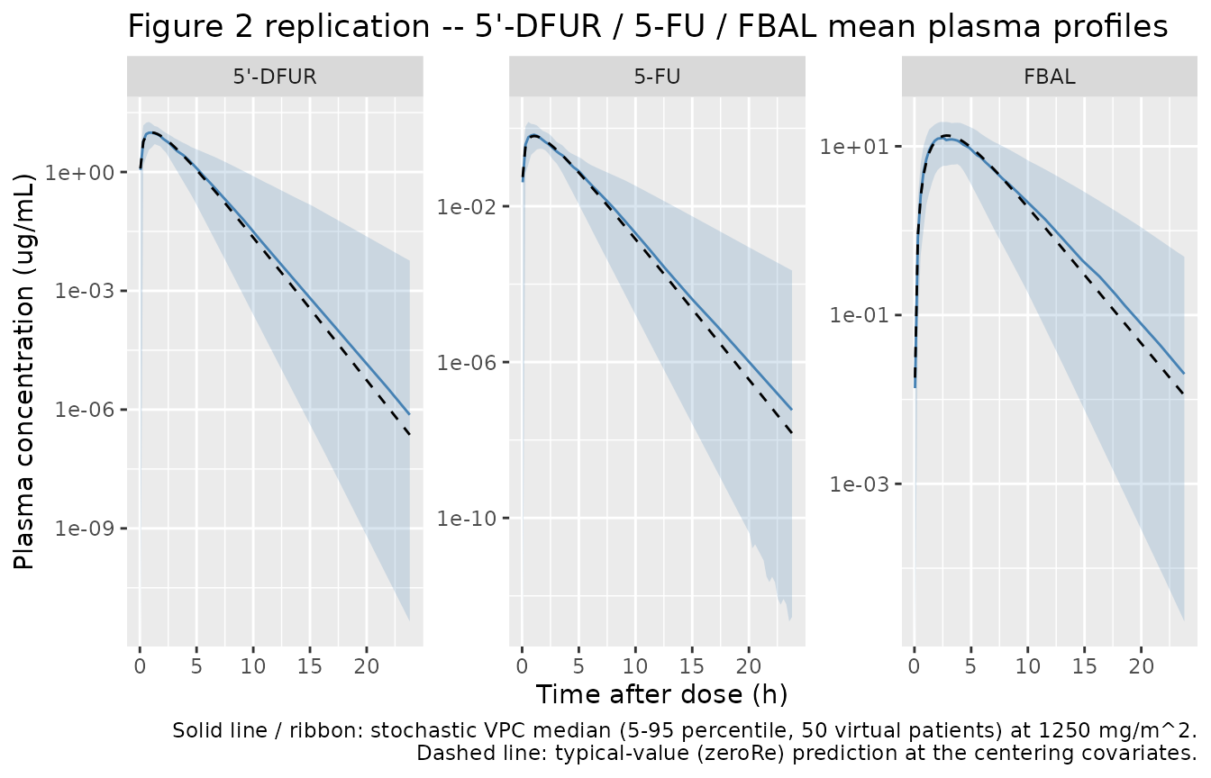
Covariate sensitivity – Table 2 reproduction
Blesch 2003 Table 2 reports the effects of multiplicative changes in ALP, CRCL, and BSA on the typical-value PK parameters and on systemic exposure. We reproduce the table here from the model file’s covariate exponents and compare against the paper’s percentages.
# Compute simulated changes for the typical patient under each Table 2
# scenario. The reference (centering) covariates are the values declared
# in the model file: ALP = 100, CRCL = 80, BSA = 1.73.
make_scenario <- function(label, ALP, CRCL, BSA) {
  ev <- rxode2::et(amt = 1250 * 1.73, cmt = "depot", time = 0)
  ev <- rxode2::et(ev, time = obs_times, cmt = "Cc_dfur")
  ev <- as.data.frame(ev)
  ev$id   <- 1L
  ev$ALP  <- ALP
  ev$CRCL <- CRCL
  ev$BSA  <- BSA
  sim_s <- rxode2::rxSolve(mod_typ, events = ev) |> as.data.frame()
  tibble::tibble(
    scenario = label,
    auc_5fu  = pracma::trapz(sim_s$time, sim_s$Cc_5fu),
    auc_fbal = pracma::trapz(sim_s$time, sim_s$Cc_fbal),
    cmax_fbal = max(sim_s$Cc_fbal, na.rm = TRUE)
  )
}
if (!requireNamespace("pracma", quietly = TRUE)) {
  # Simple trapezoidal helper as a fallback
  pracma_trapz <- function(x, y) sum(diff(x) * (head(y, -1) + tail(y, -1)) / 2)
} else {
  pracma_trapz <- pracma::trapz
}

# Re-implement using the fallback uniformly.
make_scenario <- function(label, ALP, CRCL, BSA) {
  ev <- rxode2::et(amt = 1250 * 1.73, cmt = "depot", time = 0)
  ev <- rxode2::et(ev, time = obs_times, cmt = "Cc_dfur")
  ev <- as.data.frame(ev)
  ev$id   <- 1L
  ev$ALP  <- ALP
  ev$CRCL <- CRCL
  ev$BSA  <- BSA
  sim_s <- rxode2::rxSolve(mod_typ, events = ev) |> as.data.frame()
  tibble::tibble(
    scenario  = label,
    auc_5fu   = pracma_trapz(sim_s$time, sim_s$Cc_5fu),
    auc_fbal  = pracma_trapz(sim_s$time, sim_s$Cc_fbal),
    cmax_fbal = max(sim_s$Cc_fbal, na.rm = TRUE)
  )
}

scenarios <- dplyr::bind_rows(
  make_scenario("Reference (ALP=100, CRCL=80, BSA=1.73)", 100, 80,   1.73),
  make_scenario("ALP x 2 (200)",                          200, 80,   1.73),
  make_scenario("ALP x 5 (500)",                          500, 80,   1.73),
  make_scenario("CRCL x 0.5 (40)",                        100, 40,   1.73),
  make_scenario("BSA x 1.3 (2.249)",                      100, 80,   2.249)
)
#> ℹ omega/sigma items treated as zero: 'etalka', 'etaltlag', 'etalvc_dfur', 'etalcl_dfur', 'etalcl_5fu', 'etalvc_fbal', 'etalcl_fbal'
#> ℹ omega/sigma items treated as zero: 'etalka', 'etaltlag', 'etalvc_dfur', 'etalcl_dfur', 'etalcl_5fu', 'etalvc_fbal', 'etalcl_fbal'
#> ℹ omega/sigma items treated as zero: 'etalka', 'etaltlag', 'etalvc_dfur', 'etalcl_dfur', 'etalcl_5fu', 'etalvc_fbal', 'etalcl_fbal'
#> ℹ omega/sigma items treated as zero: 'etalka', 'etaltlag', 'etalvc_dfur', 'etalcl_dfur', 'etalcl_5fu', 'etalvc_fbal', 'etalcl_fbal'
#> ℹ omega/sigma items treated as zero: 'etalka', 'etaltlag', 'etalvc_dfur', 'etalcl_dfur', 'etalcl_5fu', 'etalvc_fbal', 'etalcl_fbal'

ref <- scenarios[1, ]
sens <- scenarios |>
  dplyr::mutate(
    pct_change_5fu_auc   = round(100 * (auc_5fu   / ref$auc_5fu   - 1), 1),
    pct_change_fbal_auc  = round(100 * (auc_fbal  / ref$auc_fbal  - 1), 1),
    pct_change_fbal_cmax = round(100 * (cmax_fbal / ref$cmax_fbal - 1), 1)
  ) |>
  dplyr::select(scenario,
                `5-FU AUC % change` = pct_change_5fu_auc,
                `FBAL AUC % change` = pct_change_fbal_auc,
                `FBAL Cmax % change` = pct_change_fbal_cmax)

knitr::kable(
  sens,
  caption = "Simulated covariate sensitivity. Compare against Blesch 2003 Table 2: ALP x 2 -> +12% 5-FU AUC; ALP x 5 -> +31%; CRCL x 0.5 -> +53% FBAL AUC and +41% FBAL Cmax; BSA x 1.3 -> -19% FBAL Cmax."
)| scenario | 5-FU AUC % change | FBAL AUC % change | FBAL Cmax % change |
|---|---|---|---|
| Reference (ALP=100, CRCL=80, BSA=1.73) | 0.0 | 0.0 | 0.0 |
| ALP x 2 (200) | 12.4 | 0.0 | 0.0 |
| ALP x 5 (500) | 31.3 | 0.0 | 0.0 |
| CRCL x 0.5 (40) | 0.0 | 53.0 | 40.7 |
| BSA x 1.3 (2.249) | 0.0 | -0.1 | -11.2 |
PKNCA validation
PKNCA is run separately for each of the three analytes. The treatment
grouping variable is analyte (one entry per analyte) so
per-analyte NCA summaries can be compared head-to-head.
sim_nca_dfur <- sim |>
  dplyr::filter(!is.na(Cc_dfur)) |>
  dplyr::transmute(id, time, Cc = Cc_dfur, treatment = "5'-DFUR")

# Time-zero anchor (extravascular Cc=0 before dose).
sim_nca_dfur <- dplyr::bind_rows(
  sim_nca_dfur,
  sim_nca_dfur |> dplyr::distinct(id, treatment) |>
    dplyr::mutate(time = 0, Cc = 0)
) |>
  dplyr::distinct(id, treatment, time, .keep_all = TRUE) |>
  dplyr::arrange(id, treatment, time)

dose_df <- events |>
  dplyr::filter(evid == 1) |>
  dplyr::transmute(id, time, amt, treatment = "5'-DFUR")

conc_obj_dfur <- PKNCA::PKNCAconc(
  sim_nca_dfur, Cc ~ time | treatment + id,
  concu = "ug/mL", timeu = "h"
)
dose_obj_dfur <- PKNCA::PKNCAdose(
  dose_df, amt ~ time | treatment + id,
  doseu = "mg"
)

intervals <- data.frame(
  start       = 0,
  end         = Inf,
  cmax        = TRUE,
  tmax        = TRUE,
  aucinf.obs  = TRUE,
  half.life   = TRUE
)

nca_dfur <- PKNCA::pk.nca(PKNCA::PKNCAdata(conc_obj_dfur, dose_obj_dfur,
                                           intervals = intervals))
knitr::kable(summary(nca_dfur),
caption = "5'-DFUR simulated NCA (single oral dose, 1250 mg/m^2).")| Interval Start | Interval End | treatment | N | Cmax (ug/mL) | Tmax (h) | Half-life (h) | AUCinf,obs (h*ug/mL) |
|---|---|---|---|---|---|---|---|
| 0 | Inf | 5’-DFUR | 50 | 10.5 [41.7] | 1.05 [0.300, 2.55] | 1.04 [0.504] | 29.5 [29.4] |
sim_nca_5fu <- sim |>
  dplyr::filter(!is.na(Cc_5fu)) |>
  dplyr::transmute(id, time, Cc = Cc_5fu, treatment = "5-FU")

sim_nca_5fu <- dplyr::bind_rows(
  sim_nca_5fu,
  sim_nca_5fu |> dplyr::distinct(id, treatment) |>
    dplyr::mutate(time = 0, Cc = 0)
) |>
  dplyr::distinct(id, treatment, time, .keep_all = TRUE) |>
  dplyr::arrange(id, treatment, time)

dose_df_5fu <- dose_df |> dplyr::mutate(treatment = "5-FU")
conc_obj_5fu <- PKNCA::PKNCAconc(
  sim_nca_5fu, Cc ~ time | treatment + id,
  concu = "ug/mL", timeu = "h"
)
#> Warning in assert_conc(conc, any_missing_conc = any_missing_conc): Negative
#> concentrations found
dose_obj_5fu <- PKNCA::PKNCAdose(
  dose_df_5fu, amt ~ time | treatment + id,
  doseu = "mg"
)
nca_5fu <- PKNCA::pk.nca(PKNCA::PKNCAdata(
  conc_obj_5fu, dose_obj_5fu, intervals = intervals
))
#> Warning in assert_conc(conc = conc): Negative concentrations found
#> Warning in assert_conc(conc = conc): Negative concentrations found
#> Warning in assert_conc(conc = conc): Negative concentrations found
#> Warning in assert_conc(conc = conc): Negative concentrations found
#> Warning in assert_conc(conc = conc): Negative concentrations found
#> Warning in assert_conc(conc = conc): Negative concentrations found
#> Warning in log(data$conc): NaNs produced
#> Warning in assert_conc(conc, any_missing_conc = any_missing_conc): Negative
#> concentrations found
#> Warning in log(conc.2/conc.1): NaNs produced
knitr::kable(summary(nca_5fu),
caption = "5-FU simulated NCA.")| Interval Start | Interval End | treatment | N | Cmax (ug/mL) | Tmax (h) | Half-life (h) | AUCinf,obs (h*ug/mL) |
|---|---|---|---|---|---|---|---|
| 0 | Inf | 5-FU | 50 | 0.693 [56.4] | 1.05 [0.300, 2.55] | 1.04 [0.504] | 1.94 [30.0], n=49 |
sim_nca_fbal <- sim |>
  dplyr::filter(!is.na(Cc_fbal)) |>
  dplyr::transmute(id, time, Cc = Cc_fbal, treatment = "FBAL")

sim_nca_fbal <- dplyr::bind_rows(
  sim_nca_fbal,
  sim_nca_fbal |> dplyr::distinct(id, treatment) |>
    dplyr::mutate(time = 0, Cc = 0)
) |>
  dplyr::distinct(id, treatment, time, .keep_all = TRUE) |>
  dplyr::arrange(id, treatment, time)

dose_df_fbal <- dose_df |> dplyr::mutate(treatment = "FBAL")
conc_obj_fbal <- PKNCA::PKNCAconc(
  sim_nca_fbal, Cc ~ time | treatment + id,
  concu = "ug/mL", timeu = "h"
)
dose_obj_fbal <- PKNCA::PKNCAdose(
  dose_df_fbal, amt ~ time | treatment + id,
  doseu = "mg"
)
nca_fbal <- PKNCA::pk.nca(PKNCA::PKNCAdata(
  conc_obj_fbal, dose_obj_fbal, intervals = intervals
))
knitr::kable(summary(nca_fbal),
caption = "FBAL simulated NCA.")| Interval Start | Interval End | treatment | N | Cmax (ug/mL) | Tmax (h) | Half-life (h) | AUCinf,obs (h*ug/mL) |
|---|---|---|---|---|---|---|---|
| 0 | Inf | FBAL | 50 | 13.0 [33.5] | 2.80 [1.30, 6.05] | 2.08 [0.824] | 77.2 [43.6] |
Comparison against published exposures
Blesch 2003 does not tabulate population mean / median NCA values
directly; Figure 2 shows mean plasma concentration time curves at 1250
mg/m^2 but the AUC and Cmax point estimates per analyte are not listed
in the review text. As a sanity check we compare the simulated
typical-value (zeroRe) AUC against the analytic apparent-clearance
identity AUC_inf = Dose / CL_x_apparent and the simulated
typical-value Cmax against direct calculation from the time grid.
dose_mg <- 1250 * 1.73

analytic <- tibble::tibble(
  Analyte           = c("5'-DFUR", "5-FU", "FBAL"),
  `AUC_inf analytic (ug*h/mL)` =
    c(dose_mg / 75.8, dose_mg / 1190, dose_mg / 27.5),
  `AUC_inf simulated typical (ug*h/mL)` =
    c(
      pracma_trapz(sim_typ$time, sim_typ$Cc_dfur),
      pracma_trapz(sim_typ$time, sim_typ$Cc_5fu),
      pracma_trapz(sim_typ$time, sim_typ$Cc_fbal)
    ),
  `Cmax simulated typical (ug/mL)` =
    c(max(sim_typ$Cc_dfur), max(sim_typ$Cc_5fu), max(sim_typ$Cc_fbal))
)

knitr::kable(
  analytic,
  digits = c(0, 2, 2, 3),
  caption = "Analytic AUC = Dose / CL_x_apparent vs simulated typical-value AUC (single 2162.5 mg oral dose). The simulated AUC was integrated over 0-24 h on the simulation time grid, so it underestimates AUC_inf for the slowly-eliminated FBAL whose terminal phase extends beyond 24 h."
)| Analyte | AUC_inf analytic (ug*h/mL) | AUC_inf simulated typical (ug*h/mL) | Cmax simulated typical (ug/mL) |
|---|---|---|---|
| 5’-DFUR | 28.53 | 28.38 | 9.964 |
| 5-FU | 1.82 | 1.81 | 0.635 |
| FBAL | 78.64 | 78.60 | 13.406 |
Assumptions and deviations
- Covariate centering values are not paper-derived. Blesch 2003 does not tabulate the population’s baseline medians for ALP, CRCL, or BSA (those numeric distributions live in the cited Phase III source publications, Hoff 2001 [10] and Van Cutsem 2001 [11], which are not on disk for this extraction). The model file declares ALP = 100 U/L, CRCL = 80 mL/min/1.73 m^2, BSA = 1.73 m^2 as the centering values applied in the multiplicative power covariate effects on CL2/F, CL3/F, and V3/F. These are clinically reasonable medians for an advanced-colorectal-cancer cohort but are not from the source paper itself. Users wishing to centre on a different reference need only redivide the covariate column by their preferred reference value (the effect coefficients -0.169 / +0.615 / +0.394 / +0.812 are paper-derived from Table 1 and do not depend on the centering choice).
-
CRCL assay assumption. Blesch 2003 names the
covariate “CLCR” without stating the renal-function assay used;
era-typical for cancer popPK is Cockcroft-Gault in raw mL/min. We
register the covariate as
CRCL(canonical, mL/min/1.73 m^2) for naming consistency with the rest of nlmixr2lib, but downstream users who feed raw mL/min CrCl values into the model should be aware of the implicit BSA normalisation in the reference. -
TLAG and its inter-individual variability are essentially
unidentified. Table 1 reports TV TLAG = 5.52e-4 h (about 2
seconds) with an ISV of 49,498% CV (omega^2 ~ 12.4) – the absorption lag
parameter and its variance were both estimated but the magnitudes
indicate the data did not constrain them. The Blesch 2003 text describes
the lag as having “turned out to be the most adequate” among the
absorption models tested but the actual numeric values are not
biologically meaningful. The model file encodes the published values
verbatim; simulations should use
zeroRe()for typical-value plotting (as done above) or pre-clamp the TLAG random effect to a reasonable magnitude (e.g. CV <= 100%) for stochastic VPCs. - Inter-occasion variability on KA and TLAG is not represented. The Phase II breast-cancer cohort (Reigner 1999 [20]) supported the inclusion of an IOV term on both KA and TLAG (363-unit OFV drop). The static nlmixr2 model file does not represent IOV; downstream users that need cycle-to-cycle absorption variability should add an occasion-specific eta in their simulation harness.
-
Residual-error correlation (0.77) between 5’-DFUR and 5-FU
is not encoded. Table 1 reports the correlation between
residual epsilons for 5’-DFUR and 5-FU as 0.77 (SE 0.0435). nlmixr2’s
residual-error syntax in
model()does not directly support cross-output residual covariances, so the three proportional SDs (propSd_dfur,propSd_5fu,propSd_fbal) are independent here. The impact is on individual-level prediction intervals (the published model treats consecutive metabolite measurements as having correlated noise); population-level predictions are unaffected. - Extensive-sampling residual error chosen as the primary value. Table 1 reports a two-level residual error per analyte (extensive / sparse): 39%/51% for 5’-DFUR, 58%/76% for 5-FU, 34%/44% for FBAL. The model file uses the extensive-sampling estimates (the typical case for any density-rich dataset); users running sparse-sample-only simulations may wish to substitute the higher sparse values in their workflow.
- FBAL residual via tau parameterisation. Blesch 2003 estimated the FBAL residual variance as sigma_3^2 = (tau * sigma_dfur)^2 with tau = 0.767 (SE 0.121) fixed-effects parameter. The model file encodes the resulting %CV (34% extensive) directly rather than the derivation through tau; the directly tabulated 34% from Table 1 is used as the authoritative value (the implied 0.767 * 0.39 = 30% shows a small discrepancy with the table that is likely either rounding or a separate residual-variance baseline used during estimation).
- 5-FU volume V2 fixed at 17.8 L from external literature. Table 1 marks V2 as “TV fixed, no ISV” and the text identifies the value as literature (Heggie 1987). No ISV is estimated for V2; the identifiability sensitivity analysis showed V2 was not informative for the model, so a literature-derived fixed value is used.
- PBPK model out of scope. Blesch 2003 also describes a five-organ PBPK model (GI, blood, liver, tumour, non-eliminating tissues) for capecitabine + the three downstream-of-5’-DFCR metabolites. The PBPK parameter values are referenced from Tsukamoto et al. 2001 [reference 30 in Blesch 2003] which is not on disk for this extraction, and the PBPK section of Blesch 2003 itself reports parameter values only in narrative form rather than in a tabulated form suitable for extraction. Only the popPK model “CAP7440” (Table 1) is implemented here. The conceptual simulations, Phase I logistic-regression DLT models, and the Phase III concentration-effect analyses are likewise out of scope for an nlmixr2 popPK extraction.
- Apparent oral clearance convention. All clearances and volumes are reported as oral apparent values (CL/F, V/F). The model uses these directly in the ODEs: a clearance of 1190 L/h on the 5-FU compartment means the entire mass flux entering the 5-FU pool from 5’-DFUR is multiplied by 1190 / V_5-FU per hour, with the implicit assumption that the apparent-clearance values absorb both the molar-conversion stoichiometry and the upstream bioavailability / formation fractions. This is the same convention used in Urien_2005_capecitabine and in the parent Blesch et al. NONMEM control stream.