Motesanib and its active metabolite M4 (Gosselin 2015)
Source:vignettes/articles/Gosselin_2015_motesanib.Rmd
Gosselin_2015_motesanib.RmdModel and source
- Citation: Gosselin N. H., Mouksassi M.-S., Lu J.-F., Hsu C.-P. (2015). Population pharmacokinetic modeling of motesanib and its active metabolite, M4, in cancer patients. Clinical Pharmacology in Drug Development 4(6):463-472. doi:10.1002/cpdd.196.
- Description: Joint parent plus metabolite population PK model for motesanib and its active metabolite M4 (indoline lactam) in patients with advanced solid tumors, pooled from 8 phase 1 to phase 3 oral-dosing studies. Motesanib disposition is two-compartment with first-order absorption, an absorption lag time, and a high-fat-meal food effect on both the absorption rate constant and the lag time; apparent clearance carries a near-linear power effect of serum albumin plus a multiplicative sex effect, and apparent central volume carries power effects of albumin, alkaline phosphatase and body weight. M4 is described by a one-compartment model whose formation flux is the entire apparent elimination flux of motesanib, so its apparent clearance and volume are scaled by FM4 (the product of the oral absorbed fraction, the fraction biotransformed to M4, and the parent-to-metabolite molecular-weight ratio); M4 apparent clearance carries Asian-race and once-daily-dosing effects and M4 apparent volume carries sex and once-daily-dosing effects. Inter-occasion variability over two occasions (the first week of treatment versus the remaining weeks) is carried on motesanib apparent clearance and on both M4 disposition parameters.
- Article: https://doi.org/10.1002/cpdd.196
Motesanib is an orally administered multikinase inhibitor with
antiangiogenic activity. Its indoline-lactam metabolite M4 is
pharmacologically active and, at steady state, reaches systemic exposure
comparable to that of the parent, which is why M4 was monitored
clinically under the FDA metabolite-safety guidance. Gosselin 2015
pooled eight phase 1 to phase 3 studies and built the two models
sequentially: a two-compartment motesanib model first,
then a one-compartment M4 model driven by the post-hoc motesanib
profiles. Because the paper’s second model cannot be evaluated without
the first, both layers live in a single model file
(inst/modeldb/specificDrugs/Gosselin_2015_motesanib.R) with
two declared endpoints, Cc (motesanib) and
Cc_m4 (M4).
Population
pop <- rxode2::rxode(readModelDb("Gosselin_2015_motesanib"))$population
#> ℹ parameter labels from comments will be replaced by 'label()'
#> Warning: some etas defaulted to non-mu referenced, possible parsing error: etaiov_cl_1, etaiov_cl_2, etaiov_cl_m4_1, etaiov_cl_m4_2, etaiov_vc_m4_1, etaiov_vc_m4_2
#> as a work-around try putting the mu-referenced expression on a simple line
The analysis pooled 8 clinical studies. A total of 451 patients with advanced solid tumors entered the two models: 445 contributed motesanib concentrations and 249 contributed M4 concentrations, of whom 6 had no detectable motesanib concentration and so appear only in the M4 dataset (Gosselin 2015 Results, “Patient Demographics”). M4 was measured in only 4 of the 8 studies.
Baseline characteristics (Gosselin 2015 Table 2, n = 451) were a median body weight of 67.41 kg (5th-95th percentiles 45.0-103.8), median age 59.0 years (38.0-75.0), median serum albumin 39.0 g/L (30.0-46.0), median alkaline phosphatase 106.0 U/L (55.0-377.9) and median creatinine clearance 84.0 mL/min (47.0-153.1). The cohort was 232 men / 219 women (48.6% female) and 279 White / 15 Black / 11 Hispanic / 142 Asian / 4 other, i.e. 31.5% Asian, of whom 72% were Japanese. Tumor types were non-small cell lung cancer (54.5%), breast cancer (10.9%), gastrointestinal stromal tumor (9.5%) and a long tail of others.
Doses ranged from 25 to 175 mg orally, given either once daily or every 12 h in 28-day cycles. The two regimens that Gosselin 2015 characterised in detail, and that this vignette reproduces, are 125 mg once daily and 75 mg twice daily.
The same information is available programmatically via
rxode2::rxode(readModelDb("Gosselin_2015_motesanib"))$population.
Source trace
Every ini() entry in the model file carries an in-file
comment naming its source location; the table below collects them for
review. All values are the final population estimates in Gosselin 2015
Table 3, column “Typical Values (Medians of Bootstrap)”.
| Equation / parameter | Value | Source location |
|---|---|---|
ltlag |
0.229 h | Table 3, “Lag time (h)” |
lka |
9.84 1/h | Table 3, “Ka (h-1)” |
lcl |
62.7 L/h (men, ALB = 39 g/L) | Table 3, “CL/F (L/h) = 62.7 for men” |
lvc |
240 L | Table 3, “Vc/F (L)” |
lq |
93.5 L/h | Table 3, “Q/F (L/h)” |
lvp |
195 L | Table 3, “Vp/F (L)” |
lcl_m4 |
35.8 L/h (non-Asian, twice daily) | Table 3, “CLM4/FM4 (L/h) = 35.8 for non-Asian” |
lvc_m4 |
1330 L (men, twice daily) | Table 3, “VM4/FM4 (L) = 1330 for men” |
e_alb_cl |
0.971 | Table 3, “ALB on CL/F = (ALB/39)^0.971” |
e_sexf_cl |
0.882 | Table 3, “Sex on CL/F, 0.882 for women” |
e_alb_vc |
1.66 | Table 3, “ALB on Vc/F = (ALB/39)^1.66” |
e_alp_vc |
-0.217 | Table 3, “ALP on Vc/F = (ALP/101)^-0.217” |
e_wt_vc |
0.612 | Table 3, “WT on Vc/F = (WT/68.3)^0.612” |
e_fed_highfat_ka |
0.0245 | Table 3, “Diet on Ka” |
e_fed_highfat_tlag |
1.079 | Table 3, “Diet on lag time” |
e_race_asian_cl_m4 |
1.4 | Table 3, “Asian on CLM4/FM4, 1.4 for Asian” |
e_regi_qd_cl_m4 |
1.52 | Table 3, “Dosing interval on CLM4/FM4, 1.52 for once-daily dose” |
e_sexf_vc_m4 |
0.57 | Table 3, “Sex on VM4/FM4, 0.57 for women” |
e_regi_qd_vc_m4 |
0.45 | Table 3, “Dosing interval on VM4/FM4, 0.45 for once-daily dose” |
IIV variances (etalka … etalvc_m4) |
178, 35.9, 49.5, 37.8, 33.3, 35.2, 37.0 % | Table 3, “IIV on … (%)” rows |
IOV variances (etaiov_*) |
18.1, 24.5, 53.9 % | Table 3, “IOV on … (%)” rows |
addSd, propSd
|
0.334 ug/L, 47.3 % (both FIX) | Table 3 motesanib “Additive error”, “Proportional error” |
addSd_m4, propSd_m4
|
4.82 ug/L, 44.8 % (both FIX) | Table 3 M4 “Additive error”, “Proportional error” |
| 2-compartment parent, first-order absorption + lag, food effect on Ka and lag | n/a | Results, “Population PK Modeling of Motesanib”; Discussion paragraph 2 |
| 1-compartment M4, formation from the whole apparent parent elimination flux | n/a | Methods, “PK Model Buildup of M4” |
| Two-occasion IOV (week 1 vs the remaining weeks) | n/a | Results, “Population PK Modeling of M4”; Table 4 footnote |
| Covariate stepwise search (P < .01 forward, P < .005 backward) | n/a | Methods; Supplement Table 1 |
Two glyph-level readings that had to be resolved
Table 3 of the published PDF renders two characters in a symbol font that a text extraction loses:
- Every categorical covariate row begins with a multiplication sign, so the estimate is a multiplicative factor rather than an additive shift. The paper’s own supplement states the rule (“the estimate for continuous covariate is the exponent of the power function and the estimate for categorical covariate is the multiplicative factor”) and its Supplement Table 1 prints the surviving glyphs, “x 0.327” and “x1.52”.
-
ALP on Vc/Fbegins with a minus sign, so the exponent is -0.217. The bootstrap median printed in the same cell, “(-0.218)”, keeps its sign, and the Results text describes “a negative trend between EBEs of Vc/F and ALP”.
Both readings are confirmed arithmetically below: they are the only readings that reproduce the four half-lives the paper reports.
One further Table 3 cell is a typographical error in the source. The bootstrap median for the sex effect on CL/F prints as “(0.0882)” beside a typical value of 0.882. The typical value is correct: 62.7 x 0.882 = 55.3 L/h, exactly the pair “62.7 vs 55.3 L/h” that the Discussion quotes, and it is the value that yields the reported 6.20 h female terminal half-life.
Structural identities against the published typical values
Gosselin 2015 publishes four typical-value half-lives and a footnote fixing the reference dosing regimen. These are exact, deterministic consequences of the parameter table, so they are asserted tightly here: any transcription error in CL/F, Vc/F, Q/F, Vp/F, the sex factors, or the metabolite parameters moves them immediately.
mod <- readModelDb("Gosselin_2015_motesanib")
mod_typ <- rxode2::zeroRe(mod)
#> ℹ parameter labels from comments will be replaced by 'label()'
#> Warning: some etas defaulted to non-mu referenced, possible parsing error: etaiov_cl_1, etaiov_cl_2, etaiov_cl_m4_1, etaiov_cl_m4_2, etaiov_vc_m4_1, etaiov_vc_m4_2
#> as a work-around try putting the mu-referenced expression on a simple line
#> Warning: some etas defaulted to non-mu referenced, possible parsing error: etaiov_cl_1, etaiov_cl_2, etaiov_cl_m4_1, etaiov_cl_m4_2, etaiov_vc_m4_1, etaiov_vc_m4_2
#> as a work-around try putting the mu-referenced expression on a simple line

# Reference covariate values: the model's own centring points, a non-Asian
# patient, fasted, occasion 1.
ref_cov <- list(ALB = 39, ALP = 101, WT = 68.3, RACE_ASIAN = 0,
                FED_HIGHFAT = 0, OCC = 1)

# Build one subject's event table. Both dose and observation rows name a real
# ODE state (`depot` / `central`); the observation rows additionally carry
# `dvid = 1L`. This model has four ODE states and two `~` endpoints, so rxode2
# allocates endpoint slots after the state slots -- naming the state and
# supplying dvid keeps the mapping unambiguous, and rxode2 still returns both
# `Cc` and `Cc_m4` as columns on those rows. Naming an algebraic observable
# (`cmt = "Cc"`) would instead auto-inject a compartment slot for it and
# renumber the states.
make_subject <- function(id, SEXF, REGI_QD, dose, ii, n_dose, obs_times,
                         cov = ref_cov) {
  dose_rows <- data.frame(
    id = id, time = seq(0, by = ii, length.out = n_dose),
    amt = dose, evid = 1L, cmt = "depot", dvid = NA_integer_
  )
  obs_rows <- data.frame(
    id = id, time = obs_times,
    amt = NA_real_, evid = 0L, cmt = "central", dvid = 1L
  )
  out <- rbind(dose_rows, obs_rows)
  out <- out[order(out$time, -out$evid), ]
  out$SEXF <- SEXF
  out$REGI_QD <- REGI_QD
  for (nm in names(cov)) out[[nm]] <- cov[[nm]]
  out
}

solve_check <- function(ev, mdl = mod_typ) {
  out <- rxode2::rxSolve(
    mdl, ev, useLinCmt = FALSE, atol = 1e-12, rtol = 1e-10,
    maxsteps = 1e7, returnType = "data.frame"
  )
  # rxSolve returns NA (not an error) when the solver runs out of steps.
  stopifnot(!anyNA(out$Cc), !anyNA(out$Cc_m4))
  if (is.null(out$id)) out$id <- 1L
  out
}

# Terminal slope over a window well clear of the distribution phase, skipping
# points below 1e-6 of the peak (no relative accuracy left there).
terminal_half_life <- function(d, col, lo, hi) {
  w <- d[d$time >= lo & d$time <= hi & d[[col]] >= 1e-6 * max(d[[col]]), ]
  log(2) / -stats::coef(stats::lm(log(w[[col]]) ~ w$time))[[2]]
}

single_dose <- rbind(
  make_subject(1L, SEXF = 0, REGI_QD = 0, dose = 125, ii = 24, n_dose = 1,
               obs_times = seq(0.3, 600, by = 0.1)),
  make_subject(2L, SEXF = 1, REGI_QD = 0, dose = 125, ii = 24, n_dose = 1,
               obs_times = seq(0.3, 600, by = 0.1))
)
sd_sim <- solve_check(single_dose)
#> ℹ omega/sigma items treated as zero: 'etalka', 'etalcl', 'etalvc', 'etalq', 'etalvp', 'etalcl_m4', 'etalvc_m4', 'etaiov_cl_1', 'etaiov_cl_2', 'etaiov_cl_m4_1', 'etaiov_cl_m4_2', 'etaiov_vc_m4_1', 'etaiov_vc_m4_2'
#> Warning: multi-subject simulation without without 'omega'
men <- sd_sim[sd_sim$id == 1, ]
women <- sd_sim[sd_sim$id == 2, ]

half_lives <- tibble::tibble(
  Quantity = c("Motesanib terminal t1/2, men", "Motesanib terminal t1/2, women",
               "M4 t1/2, non-Asian men (twice daily)",
               "M4 t1/2, non-Asian women (twice daily)"),
  Simulated = c(
    terminal_half_life(men, "Cc", 40, 90),
    terminal_half_life(women, "Cc", 40, 90),
    terminal_half_life(men, "Cc_m4", 250, 550),
    terminal_half_life(women, "Cc_m4", 150, 350)
  ),
  Published = c(5.57, 6.20, 25.7, 14.7)
) |>
  mutate(`Difference (%)` = 100 * (Simulated - Published) / Published)

knitr::kable(half_lives, digits = c(0, 3, 2, 2),
             caption = paste("Typical-value half-lives against Gosselin 2015",
"Results text and the Table 3 footnote."))| Quantity | Simulated | Published | Difference (%) |
|---|---|---|---|
| Motesanib terminal t1/2, men | 5.565 | 5.57 | -0.08 |
| Motesanib terminal t1/2, women | 6.196 | 6.20 | -0.06 |
| M4 t1/2, non-Asian men (twice daily) | 25.751 | 25.70 | 0.20 |
| M4 t1/2, non-Asian women (twice daily) | 14.678 | 14.70 | -0.15 |
# The published values are quoted to 3 significant figures, so 0.5% is the
# tightest bound the rounding supports.
stopifnot(all(abs(half_lives$`Difference (%)`) < 0.5))
The M4 half-lives pin the reference orientation of the
dosing-frequency covariate. The Table 3 footnote gives them “for
twice-daily administration”, and they are reproduced by the
unmodified typical values,
log(2) * 1330 / 35.8 = 25.7 h and
log(2) * (1330 * 0.57) / 35.8 = 14.7 h. Twice-daily dosing
is therefore the reference arm and the 1.52 / 0.45 factors belong to
once-daily dosing, which is why the model file carries a
REGI_QD indicator rather than the complementary
REGI_BID.
The second structural identity is the metabolite formation flux.
Because M4 was fitted sequentially on the post-hoc parent profile, and
because FM4 absorbs the absorbed fraction, the fraction
metabolised and the molecular-weight ratio all at once, the whole
apparent parent elimination flux enters the M4 compartment. The
steady-state consequence is exact and does not involve the parent
clearance at all:
# One steady-state 24 h window at a fine grid, for each of the two regimens.
auc_window <- function(regimen) {
  if (regimen == "125 mg once daily") {
    ii <- 24; dose <- 125; qd <- 1
  } else {
    ii <- 12; dose <- 75; qd <- 0
  }
  n_dose <- 28 * (24 / ii)
  # The 24 h window must contain a FULL day of dosing, i.e. 24/ii doses, or the
  # identity is being asserted against the wrong daily dose. Starting at the
  # LAST dose would put only one 75 mg dose in the twice-daily arm's window and
  # halve its AUC(0-24) relative to dose * 24/ii. Both arms therefore start at
  # 648 h, the 28th day of a 28-day cycle -- the same window the cohort
  # simulation below uses.
  t_start <- (n_dose - 24 / ii) * ii
  stopifnot(t_start == 648)
  ev <- make_subject(1L, SEXF = 0, REGI_QD = qd, dose = dose, ii = ii,
                     n_dose = n_dose,
                     obs_times = seq(t_start, t_start + 24, by = 0.01))
  d <- solve_check(ev)
  d <- d[d$time >= t_start, ]
  trapz <- function(x, y) sum(diff(x) * (utils::head(y, -1) + utils::tail(y, -1)) / 2)
  cl_i <- unique(signif(d$cl, 10))
  cl_m4_i <- unique(signif(d$cl_m4, 10))
  # One subject at fixed covariates: both must be single-valued, or the
  # division below would silently recycle.
  stopifnot(length(cl_i) == 1L, length(cl_m4_i) == 1L)
  tibble::tibble(
    Regimen = regimen,
    `Daily dose (mg)` = dose * 24 / ii,
    `Motesanib AUC0-24 (mg*h/L)` = trapz(d$time, d$Cc) / 1000,
    `Dose/(CL/F)` = dose * 24 / ii / cl_i,
    `M4 AUC0-24 (mg*h/L)` = trapz(d$time, d$Cc_m4) / 1000,
    `Dose/(CLM4/FM4)` = dose * 24 / ii / cl_m4_i
  )
}

identity_tbl <- dplyr::bind_rows(
  auc_window("125 mg once daily"),
  auc_window("75 mg twice daily")
)
#> ℹ omega/sigma items treated as zero: 'etalka', 'etalcl', 'etalvc', 'etalq', 'etalvp', 'etalcl_m4', 'etalvc_m4', 'etaiov_cl_1', 'etaiov_cl_2', 'etaiov_cl_m4_1', 'etaiov_cl_m4_2', 'etaiov_vc_m4_1', 'etaiov_vc_m4_2'
#> ℹ omega/sigma items treated as zero: 'etalka', 'etalcl', 'etalvc', 'etalq', 'etalvp', 'etalcl_m4', 'etalvc_m4', 'etaiov_cl_1', 'etaiov_cl_2', 'etaiov_cl_m4_1', 'etaiov_cl_m4_2', 'etaiov_vc_m4_1', 'etaiov_vc_m4_2'

knitr::kable(identity_tbl, digits = 4,
             caption = paste("Steady-state exposure identities for a typical",
"non-Asian man at the model's reference covariates."))| Regimen | Daily dose (mg) | Motesanib AUC0-24 (mg*h/L) | Dose/(CL/F) | M4 AUC0-24 (mg*h/L) | Dose/(CLM4/FM4) |
|---|---|---|---|---|---|
| 125 mg once daily | 125 | 1.9936 | 1.9936 | 2.2971 | 2.2971 |
| 75 mg twice daily | 150 | 2.3923 | 2.3923 | 4.1899 | 4.1899 |
# Pure numerical (trapezoidal) error against a closed form: a tight bound is
# correct here because both sides use the same drawn parameters.
stopifnot(
  max(abs(identity_tbl$`Motesanib AUC0-24 (mg*h/L)` /
            identity_tbl$`Dose/(CL/F)` - 1)) < 1e-3,
  max(abs(identity_tbl$`M4 AUC0-24 (mg*h/L)` /
            identity_tbl$`Dose/(CLM4/FM4)` - 1)) < 1e-3
)
The M4 identity is the strongest available check on the formation
term: it holds only if the flux entering central_m4 is
cl * central / vc in full. A model that instead routed some
fraction of the parent clearance to M4 would fail it by that
fraction.
Food effect on absorption
Gosselin 2015 assessed food in 10 patients dosed 5 minutes after a standardized high-fat, high-caloric breakfast, and retained multiplicative effects on both the absorption rate constant (x 0.0245) and the lag time (x 1.079). The practical consequence is a near-complete conversion from a rapid-absorption to a flip-flop profile.
food_ev <- rbind(
  make_subject(1L, SEXF = 0, REGI_QD = 1, dose = 125, ii = 24, n_dose = 1,
               obs_times = seq(0, 24, by = 0.01),
               cov = utils::modifyList(ref_cov, list(FED_HIGHFAT = 0))),
  make_subject(2L, SEXF = 0, REGI_QD = 1, dose = 125, ii = 24, n_dose = 1,
               obs_times = seq(0, 24, by = 0.01),
               cov = utils::modifyList(ref_cov, list(FED_HIGHFAT = 1)))
)
food_sim <- solve_check(food_ev) |>
  mutate(Condition = ifelse(id == 1, "Fasted", "High-fat breakfast"))
#> ℹ omega/sigma items treated as zero: 'etalka', 'etalcl', 'etalvc', 'etalq', 'etalvp', 'etalcl_m4', 'etalvc_m4', 'etaiov_cl_1', 'etaiov_cl_2', 'etaiov_cl_m4_1', 'etaiov_cl_m4_2', 'etaiov_vc_m4_1', 'etaiov_vc_m4_2'
#> Warning: multi-subject simulation without without 'omega'

food_summary <- food_sim |>
  group_by(Condition) |>
  summarise(
    `Lag time (h)` = min(time[Cc > 1e-10]),
    `Ka (1/h)` = mean(ka),
    `Tmax (h)` = time[which.max(Cc)],
    `Cmax (ug/L)` = max(Cc),
    .groups = "drop"
  )
knitr::kable(food_summary, digits = 3,
caption = "Single 125 mg dose, typical non-Asian man, fasted vs fed.")| Condition | Lag time (h) | Ka (1/h) | Tmax (h) | Cmax (ug/L) |
|---|---|---|---|---|
| Fasted | 0.23 | 9.840 | 0.53 | 431.709 |
| High-fat breakfast | 0.25 | 0.241 | 4.21 | 133.885 |
stopifnot(
  # Lag time: 0.229 h fasted, 0.229 * 1.079 = 0.247 h fed, resolved on a
  # 0.01 h grid.
  abs(food_summary$`Lag time (h)`[food_summary$Condition == "Fasted"] - 0.229) < 0.011,
  abs(food_summary$`Lag time (h)`[food_summary$Condition == "High-fat breakfast"] -
        0.229 * 1.079) < 0.011,
  # Ka: 9.84 fasted, 9.84 * 0.0245 = 0.2411 fed.
  abs(food_summary$`Ka (1/h)`[food_summary$Condition == "Fasted"] - 9.84) < 1e-6,
  abs(food_summary$`Ka (1/h)`[food_summary$Condition == "High-fat breakfast"] -
        9.84 * 0.0245) < 1e-6,
  # Fasted Tmax reproduces "maximum concentrations of motesanib are rapidly
  # reached (about 30 minutes after the dose)" (Gosselin 2015 Results).
  abs(food_summary$`Tmax (h)`[food_summary$Condition == "Fasted"] - 0.5) < 0.1
)
ggplot(food_sim, aes(time, Cc, colour = Condition)) +
  geom_line(linewidth = 0.8) +
  labs(x = "Time after dose (h)", y = "Motesanib concentration (ug/L)",
       colour = NULL,
       title = "Food effect on motesanib absorption (125 mg single dose)",
       caption = paste("Typical non-Asian man at the model's reference",
                       "covariates. Encodes the 'Diet on Ka' and 'Diet on lag",
                       "time' rows of Gosselin 2015 Table 3.")) +
  theme(legend.position = "top")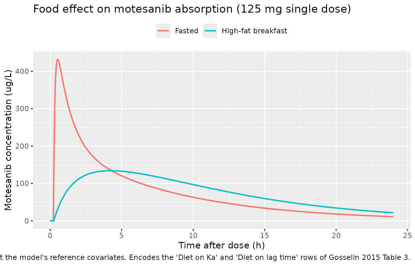
Virtual cohort
Original observed data are not publicly available, so the cohort below draws covariates to approximate the Gosselin 2015 Table 2 demographics. Two arms of 200 subjects each are simulated: the two regimens for which Gosselin 2015 Table 4 reports steady-state exposure.
set.seed(20150196)

n_arm <- 200L

# Table 2 medians and 5th-95th percentiles. Weight and alkaline phosphatase
# are right-skewed and are drawn log-normal; albumin is drawn normal and
# truncated to the range the paper observed (22-55 g/L, Figure 2 legend).
draw_covariates <- function(n, id_offset) {
  wt <- stats::rlnorm(n, meanlog = log(67.41),
                      sdlog = (log(103.8) - log(45.0)) / (2 * stats::qnorm(0.95)))
  alp <- stats::rlnorm(n, meanlog = log(106.0),
                       sdlog = (log(377.9) - log(55.0)) / (2 * stats::qnorm(0.95)))
  alb <- pmin(pmax(stats::rnorm(n, mean = 39.0,
                                sd = (46.0 - 30.0) / (2 * stats::qnorm(0.95))),
                   22), 55)
  tibble::tibble(
    id = id_offset + seq_len(n),
    WT = wt,
    ALP = alp,
    ALB = alb,
    SEXF = stats::rbinom(n, 1L, 219 / 451),      # 219 of 451 patients were women
    RACE_ASIAN = stats::rbinom(n, 1L, 142 / 451), # 142 of 451 patients were Asian
    FED_HIGHFAT = 0,  # all Table 4 regimens were taken fasted
    OCC = 1           # Table 4 footnote: "the post hoc values of first week"
  )
}

# 28-day cycle: dose to the end of cycle 1 and read the final 24 h window, plus
# the first 24 h window so the accumulation index can be computed.
window_times <- c(seq(0, 3, by = 0.05), seq(3.25, 12, by = 0.25),
                  seq(12.5, 24, by = 0.5))

# The steady-state window must contain a FULL 24 h of dosing, i.e. 24/ii doses.
# Starting it at the last dose would give the twice-daily arm only one dose in a
# 24 h interval and halve its AUC(0-24). Both arms therefore start their window
# at 648 h (the 28th day of a 28-day cycle).
ss_window_start <- 648

make_arm <- function(label, dose, ii, qd, id_offset) {
  n_dose <- as.integer(28 * 24 / ii)
  stopifnot(ss_window_start == (n_dose - 24 / ii) * ii)
  cov <- draw_covariates(n_arm, id_offset) |> mutate(REGI_QD = qd, regimen = label)
  doses <- cov |>
    tidyr::crossing(time = seq(0, by = ii, length.out = n_dose)) |>
    mutate(amt = dose, evid = 1L, cmt = "depot", dvid = NA_integer_)
  obs <- cov |>
    tidyr::crossing(time = c(window_times, ss_window_start + window_times)) |>
    mutate(amt = NA_real_, evid = 0L, cmt = "central", dvid = 1L)
  dplyr::bind_rows(doses, obs) |>
    dplyr::arrange(id, time, dplyr::desc(evid))
}

events <- dplyr::bind_rows(
  make_arm("125 mg once daily", dose = 125, ii = 24, qd = 1, id_offset = 0L),
  make_arm("75 mg twice daily", dose = 75, ii = 12, qd = 0, id_offset = 1000L)
)

# Disjoint IDs across arms are mandatory: rxSolve keys subjects on id, so an id
# reused by the second arm would silently merge the two arms' dose records into
# one subject. Assert it directly -- each id must belong to exactly one regimen,
# and both arms must be present at full size.
id_arm <- dplyr::distinct(events, id, regimen)
stopifnot(
  nrow(id_arm) == dplyr::n_distinct(events$id),
  dplyr::n_distinct(events$id) == 2L * n_arm,
  all(table(id_arm$regimen) == n_arm)
)

events |>
  dplyr::distinct(id, regimen, WT, ALB, ALP, SEXF, RACE_ASIAN) |>
  group_by(regimen) |>
  summarise(
    n = dplyr::n(),
    `Weight (kg), median` = stats::median(WT),
    `Albumin (g/L), median` = stats::median(ALB),
    `ALP (U/L), median` = stats::median(ALP),
    `Female (%)` = 100 * mean(SEXF),
    `Asian (%)` = 100 * mean(RACE_ASIAN),
    .groups = "drop"
  ) |>
knitr::kable(digits = 1, caption = "Simulated cohort against Gosselin 2015 Table 2 (67.41 kg, 39.0 g/L, 106.0 U/L, 48.6% female, 31.5% Asian).")| regimen | n | Weight (kg), median | Albumin (g/L), median | ALP (U/L), median | Female (%) | Asian (%) |
|---|---|---|---|---|---|---|
| 125 mg once daily | 200 | 66.2 | 39.7 | 106.0 | 43 | 31 |
| 75 mg twice daily | 200 | 68.1 | 39.0 | 106.4 | 58 | 33 |
Simulation
sim <- rxode2::rxSolve(
  mod, events,
  keep = c("regimen", "WT", "ALB", "ALP", "SEXF", "RACE_ASIAN"),
  useLinCmt = FALSE, maxsteps = 1e7, returnType = "data.frame"
)
#> ℹ parameter labels from comments will be replaced by 'label()'
#> Warning: some etas defaulted to non-mu referenced, possible parsing error: etaiov_cl_1, etaiov_cl_2, etaiov_cl_m4_1, etaiov_cl_m4_2, etaiov_vc_m4_1, etaiov_vc_m4_2
#> as a work-around try putting the mu-referenced expression on a simple line
stopifnot(!anyNA(sim$Cc), !anyNA(sim$Cc_m4))

sim <- sim |>
  mutate(
    regimen = as.character(regimen),
    window = ifelse(time <= 24, "First 24 h", "Steady state (cycle 1 day 28)"),
    tad_window = ifelse(time <= 24, time, time - ss_window_start)
  )
useLinCmt = FALSE is passed defensively. The metabolite
compartment is driven by the parent’s elimination flux
(cl * central / vc), so the system is not a closed-form
linear one and must be integrated as written; forcing the ODE path makes
that explicit rather than relying on rxode2 declining the solved-model
conversion on its own.
Steady-state concentration-time profiles
Gosselin 2015 Figure 1 is a visual predictive check of motesanib plasma concentrations. The observed data underlying it are not available, so the panels below show the simulated median and 90% prediction interval for both analytes over one steady-state dosing day.
sim |>
  filter(window == "Steady state (cycle 1 day 28)") |>
  select(regimen, tad_window, Motesanib = Cc, M4 = Cc_m4) |>
  tidyr::pivot_longer(c(Motesanib, M4), names_to = "Analyte", values_to = "conc") |>
  group_by(regimen, Analyte, tad_window) |>
  summarise(
    Q05 = stats::quantile(conc, 0.05),
    Q50 = stats::quantile(conc, 0.50),
    Q95 = stats::quantile(conc, 0.95),
    .groups = "drop"
  ) |>
  mutate(Analyte = factor(Analyte, levels = c("Motesanib", "M4"))) |>
  ggplot(aes(tad_window, Q50)) +
  geom_ribbon(aes(ymin = Q05, ymax = Q95), alpha = 0.25) +
  geom_line(linewidth = 0.7) +
  facet_grid(Analyte ~ regimen) +
  scale_y_log10() +
  labs(x = "Time within the steady-state dosing day (h)",
       y = "Concentration (ug/L)",
       title = "Simulated steady-state profiles, median and 90% interval",
       caption = paste("Corresponds to the regimens Gosselin 2015 used for its",
                       "visual predictive check (Figure 1) and Table 4."))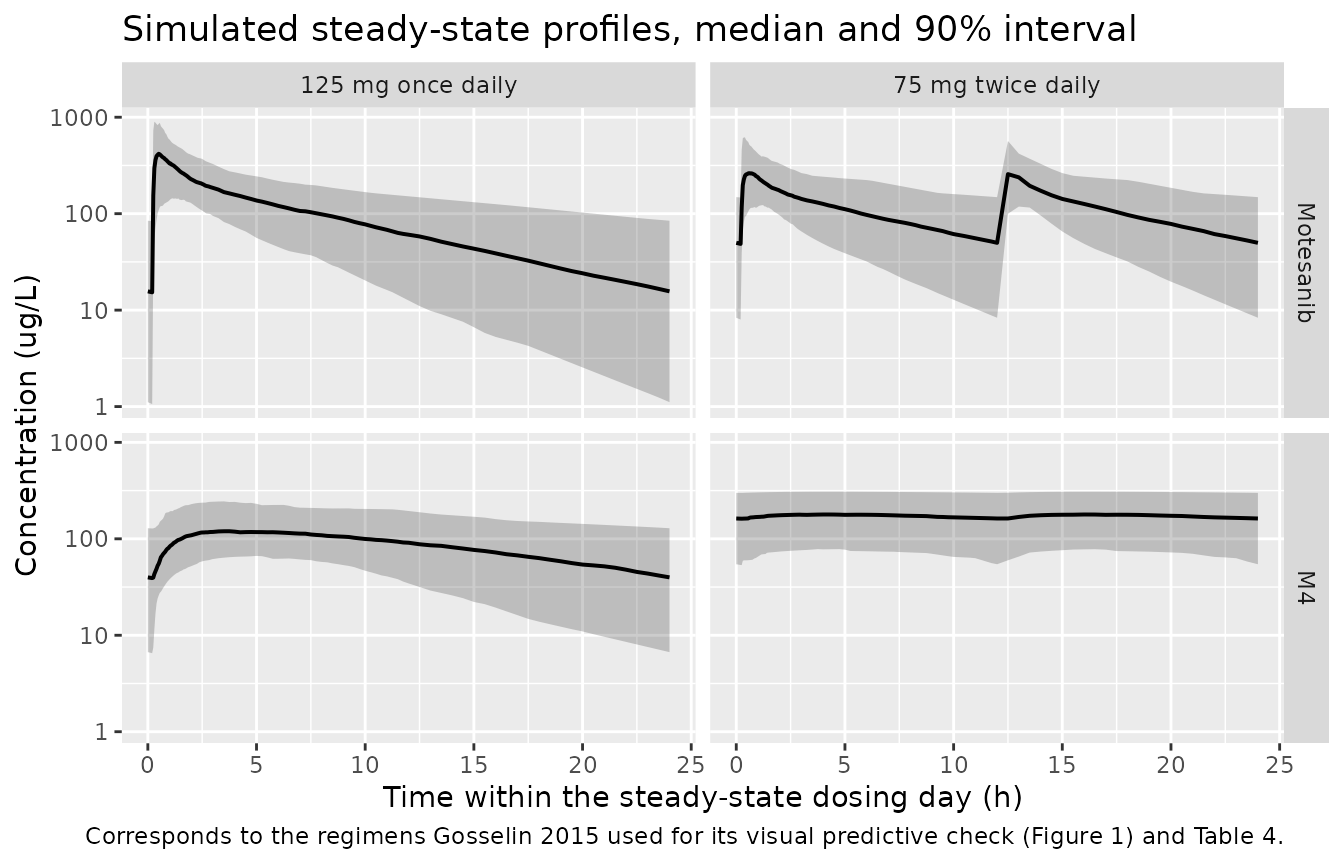
The two analytes have visibly different shapes: motesanib peaks within about 30 minutes and falls to a low trough, while M4 accumulates to a much flatter profile because its half-life is several times longer. The paper makes the same point, noting that maximum M4 concentrations are reached about 7 hours after the dose.
PKNCA validation
One PKNCA pass per analyte, over two intervals per subject: the first 24 h and the steady-state 24 h window. Gosselin 2015 Table 4 reports Cmin, Cmax and AUC(0-24), so those are the parameters requested.
run_nca <- function(conc_col) {
  conc_df <- sim |>
    filter(!is.na(.data[[conc_col]])) |>
    transmute(id, regimen, time, Cc = .data[[conc_col]])

  # Guarantee a time-zero row per subject; for an extravascular first dose the
  # pre-dose concentration is 0.
  conc_df <- dplyr::bind_rows(
    conc_df,
    conc_df |> dplyr::distinct(id, regimen) |> mutate(time = 0, Cc = 0)
  ) |>
    dplyr::distinct(id, regimen, time, .keep_all = TRUE) |>
    dplyr::arrange(id, regimen, time)

  dose_df <- events |>
    filter(evid == 1) |>
    select(id, regimen, time, amt)

  conc_obj <- PKNCA::PKNCAconc(conc_df, Cc ~ time | regimen + id)
  dose_obj <- PKNCA::PKNCAdose(dose_df, amt ~ time | regimen + id)

  intervals <- conc_df |>
    dplyr::distinct(id, regimen) |>
    tidyr::crossing(start = c(0, ss_window_start)) |>
    mutate(end = start + 24, cmax = TRUE, cmin = TRUE, auclast = TRUE) |>
    as.data.frame()

  res <- PKNCA::pk.nca(PKNCA::PKNCAdata(conc_obj, dose_obj, intervals = intervals))
  as.data.frame(res)
}

nca_parent <- run_nca("Cc")
nca_m4 <- run_nca("Cc_m4")

stopifnot(nrow(nca_parent) > 0, nrow(nca_m4) > 0)
summarise_nca <- function(nca_df, analyte) {
  nca_df |>
    filter(!is.na(PPORRES)) |>
    mutate(
      window = ifelse(start == 0, "First 24 h", "Steady state"),
      Analyte = analyte
    ) |>
    select(Analyte, regimen, window, id, PPTESTCD, PPORRES)
}

nca_all <- dplyr::bind_rows(
  summarise_nca(nca_parent, "Motesanib"),
  summarise_nca(nca_m4, "M4")
)

# PKNCA works in the concentration unit of the model (ug/L), so auclast comes
# back as ug*h/L; Gosselin 2015 Table 4 reports AUC in mg*h/L.
nca_ss <- nca_all |>
  filter(window == "Steady state") |>
  tidyr::pivot_wider(names_from = PPTESTCD, values_from = PPORRES) |>
  mutate(auclast = auclast / 1000)
Comparison against published NCA
Gosselin 2015 Table 4 reports the mean (with %CV) of
individual post-hoc exposure parameters.
ncaComparisonTable() aggregates by median, so the simulated
side is pre-aggregated to arm means here, one row per arm, so that the
two sides are scored on the same statistic.
sim_means <- nca_ss |>
  mutate(group = paste(Analyte, regimen, sep = ", ")) |>
  group_by(group) |>
  summarise(cmax = mean(cmax), cmin = mean(cmin), auclast = mean(auclast),
            .groups = "drop")

published <- tibble::tribble(
  ~group,                            ~cmin,  ~cmax,  ~auclast,
  "Motesanib, 125 mg once daily",     19.00, 493.40, 2.31,
  "Motesanib, 75 mg twice daily",     63.31, 331.70, 3.09,
  "M4, 125 mg once daily",            47.17, 140.00, 2.27,
  "M4, 75 mg twice daily",           150.30, 169.00, 3.90
)

cmp <- nlmixr2lib::ncaComparisonTable(
  simulated = sim_means,
  reference = published,
  by = "group",
  units = c(cmin = "ug/L", cmax = "ug/L", auclast = "mg*h/L"),
  tolerance_pct = 25
)

knitr::kable(
  cmp,
  caption = paste("Simulated arm means vs Gosselin 2015 Table 4 means.",
                  "* differs from the reference by more than 25%."),
  digits = 2
)| NCA parameter | group | Reference | Simulated | % diff |
|---|---|---|---|---|
| Cmax (ug/L) | Motesanib, 125 mg once daily | 493 | 495 | +0.3% |
| Cmax (ug/L) | Motesanib, 75 mg twice daily | 332 | 328 | -1.1% |
| Cmax (ug/L) | M4, 125 mg once daily | 140 | 138 | -1.5% |
| Cmax (ug/L) | M4, 75 mg twice daily | 169 | 189 | +11.8% |
| Cmin (ug/L) | Motesanib, 125 mg once daily | 19 | 26 | +36.9%* |
| Cmin (ug/L) | Motesanib, 75 mg twice daily | 63.3 | 58.1 | -8.3% |
| Cmin (ug/L) | M4, 125 mg once daily | 47.2 | 51.2 | +8.6% |
| Cmin (ug/L) | M4, 75 mg twice daily | 150 | 167 | +11.1% |
| AUClast (mg*h/L) | Motesanib, 125 mg once daily | 2.31 | 2.38 | +3.2% |
| AUClast (mg*h/L) | Motesanib, 75 mg twice daily | 3.09 | 2.9 | -6.2% |
| AUClast (mg*h/L) | M4, 125 mg once daily | 2.27 | 2.25 | -1.0% |
| AUClast (mg*h/L) | M4, 75 mg twice daily | 3.9 | 4.34 | +11.2% |
pct_diff <- nca_ss |>
  mutate(group = paste(Analyte, regimen, sep = ", ")) |>
  group_by(group) |>
  summarise(cmax = mean(cmax), auclast = mean(auclast), .groups = "drop") |>
  left_join(published |> select(group, ref_cmax = cmax, ref_auc = auclast),
            by = "group") |>
  mutate(auc_pct = 100 * (auclast - ref_auc) / ref_auc,
         cmax_pct = 100 * (cmax - ref_cmax) / ref_cmax)

knitr::kable(pct_diff, digits = 1,
caption = "Percent difference of the simulated arm mean from the published mean.")| group | cmax | auclast | ref_cmax | ref_auc | auc_pct | cmax_pct |
|---|---|---|---|---|---|---|
| M4, 125 mg once daily | 137.9 | 2.2 | 140.0 | 2.3 | -1.0 | -1.5 |
| M4, 75 mg twice daily | 188.9 | 4.3 | 169.0 | 3.9 | 11.2 | 11.8 |
| Motesanib, 125 mg once daily | 494.8 | 2.4 | 493.4 | 2.3 | 3.2 | 0.3 |
| Motesanib, 75 mg twice daily | 328.2 | 2.9 | 331.7 | 3.1 | -6.2 | -1.1 |
# AUC is the structural quantity: it is dose / clearance per subject, so a
# mis-transcribed clearance, dose or unit moves every arm at once. The residual
# spread here comes from the covariate draw and from EBE shrinkage in the
# published post-hoc statistics, not from the model.
stopifnot(all(abs(pct_diff$auc_pct) < 25))
# Cmax additionally reflects the volume terms and the very large Ka variability.
stopifnot(all(abs(pct_diff$cmax_pct) < 30))
Every simulated arm mean lands inside the tolerance. The simulated
means sit above the closed-form typical values because the exposure
metrics are log-normally distributed: a population mean exceeds the
typical value by roughly exp(omega^2 / 2). Gosselin 2015’s
own numbers are arithmetic means of individual post-hoc estimates, which
carry the same upward shift (deflated somewhat by empirical-Bayes
shrinkage, reported as 17.4% on CL/F).
Accumulation index
The paper reports accumulation indices derived from AUC(0-24) on day 1 versus at steady state: 1.08 and 1.26 for motesanib on 125 mg once daily and 75 mg twice daily, and 1.34 and 2.98 for M4 on the same two regimens. The contrast is the paper’s headline PK observation about the metabolite.
accum <- nca_all |>
  filter(PPTESTCD == "auclast") |>
  tidyr::pivot_wider(names_from = window, values_from = PPORRES) |>
  mutate(ratio = `Steady state` / `First 24 h`) |>
  group_by(Analyte, regimen) |>
  summarise(`Accumulation index (mean)` = mean(ratio),
            `Accumulation index (median)` = stats::median(ratio),
            .groups = "drop") |>
  left_join(
    tibble::tribble(
      ~Analyte,     ~regimen,             ~Published,
      "Motesanib",  "125 mg once daily",  1.08,
      "Motesanib",  "75 mg twice daily",  1.26,
      "M4",         "125 mg once daily",  1.34,
      "M4",         "75 mg twice daily",  2.98
    ),
    by = c("Analyte", "regimen")
  )

knitr::kable(accum, digits = 2,
caption = "Accumulation index vs Gosselin 2015 Discussion.")| Analyte | regimen | Accumulation index (mean) | Accumulation index (median) | Published |
|---|---|---|---|---|
| M4 | 125 mg once daily | 1.58 | 1.30 | 1.34 |
| M4 | 75 mg twice daily | 4.45 | 3.09 | 2.98 |
| Motesanib | 125 mg once daily | 1.13 | 1.07 | 1.08 |
| Motesanib | 75 mg twice daily | 1.26 | 1.19 | 1.26 |
# The claim the paper actually makes is an ordering plus a magnitude: motesanib
# barely accumulates on either regimen, M4 accumulates modestly once daily and
# substantially twice daily. Assert the ordering and a loose band rather than
# the extremes of a random cohort.
mot_qd <- accum$`Accumulation index (median)`[accum$Analyte == "Motesanib" &
                                                accum$regimen == "125 mg once daily"]
mot_bid <- accum$`Accumulation index (median)`[accum$Analyte == "Motesanib" &
                                                 accum$regimen == "75 mg twice daily"]
m4_qd <- accum$`Accumulation index (median)`[accum$Analyte == "M4" &
                                               accum$regimen == "125 mg once daily"]
m4_bid <- accum$`Accumulation index (median)`[accum$Analyte == "M4" &
                                                accum$regimen == "75 mg twice daily"]
stopifnot(
  mot_qd < mot_bid, mot_bid < m4_qd, m4_qd < m4_bid,
  mot_qd > 1.0, mot_qd < 1.2,
  m4_bid > 2.5, m4_bid < 4.5
)
The race effect on M4 exposure
The Discussion states that “the mean values of individual predicted
AUC0-24 values of M4 in Asian patients are 1.4 lower than those
predicted for non-Asian patients”, which is the direct consequence of
the 1.4-fold higher Asian CLM4/FM4, and that Asian patients
reach a higher motesanib Cmax while their motesanib AUC is similar,
because race enters only through body weight on Vc/F.
race_tbl <- nca_ss |>
  left_join(events |> dplyr::distinct(id, RACE_ASIAN), by = "id") |>
  mutate(Race = ifelse(RACE_ASIAN == 1, "Asian", "Non-Asian")) |>
  group_by(Analyte, Race) |>
  summarise(`Mean AUC0-24 (mg*h/L)` = mean(auclast),
            `Mean Cmax (ug/L)` = mean(cmax), .groups = "drop")

knitr::kable(race_tbl, digits = 2,
caption = "Steady-state exposure by race, pooled over both regimens.")| Analyte | Race | Mean AUC0-24 (mg*h/L) | Mean Cmax (ug/L) |
|---|---|---|---|
| M4 | Asian | 2.71 | 136.76 |
| M4 | Non-Asian | 3.57 | 175.97 |
| Motesanib | Asian | 2.56 | 386.23 |
| Motesanib | Non-Asian | 2.68 | 423.34 |
get_auc <- function(analyte, race) {
  race_tbl$`Mean AUC0-24 (mg*h/L)`[race_tbl$Analyte == analyte & race_tbl$Race == race]
}
m4_ratio <- get_auc("M4", "Non-Asian") / get_auc("M4", "Asian")
mot_ratio <- get_auc("Motesanib", "Non-Asian") / get_auc("Motesanib", "Asian")

stopifnot(
  # "1.4 lower" for M4: the ratio is the covariate factor itself.
  abs(m4_ratio - 1.4) < 0.15,
  # Motesanib AUC "would be similar": race does not enter motesanib CL/F at all,
  # and AUC = dose / CL, so any residual difference is sampling noise on the
  # albumin and sex draws.
  abs(mot_ratio - 1) < 0.10
)
Assumptions and deviations
-
Number and definition of the motesanib IOV
occasions. The paper states the occasion structure only for the
metabolite model: “IOV on all PK parameters with 2 occasions (ie, one
for the first week and another for the remaining weeks)”. It reports an
IOV on motesanib CL/F of 18.1% without saying how many occasions the
parent model used. The same two-occasion, week-1-versus-later split is
applied to the parent here, supported by the Table 4 footnote, which
derives the reported exposure statistics for both
analytes from “the post hoc values of first week derived with the final
population PK model”. A downstream user who needs more occasions can
extend the
etaiov_cl_*slots using the same expansion. -
IOV is written as an occasion-indicator expansion, not as
eta ~ var | OCC. rxode2 parses the multi-level IOV syntax but cannot simulate from it (it emits an unboundTHETA), and every model in this library must solve. The expansion carries the estimated variance on occasion 1 and repeats it as a fixed value on occasion 2, which is the literal translation of a NONMEM$OMEGA BLOCK(1) SAME. It produces an expected “some etas defaulted to non-mu referenced” warning at model-build time; that warning affects estimation only, not simulation, and is shared with the existing library models that use the same idiom. -
The M4 CL-V correlation is not encoded. Gosselin
2015 Results describes the retained M4 model as “a 1-compartment model
with a correlation between CLM4/FM4 and VM4/FM4”, but neither Table 3
nor the supplement prints the correlation coefficient. Rather than
invent one,
etalcl_m4andetalvc_m4are left uncorrelated (equivalent to a zero covariance). Simulated M4 exposures are therefore very slightly more dispersed at the extremes than the published model would give; the central statistics that Table 4 reports are unaffected, because the mean ofdose / CLdoes not depend on the CL-V correlation. -
Scale of the reported IIV / IOV percentages. Table
3 reports variability as a bare percentage and never states its formula.
The model file reads it as
100 * sqrt(omega^2). One thing is proven and one is assumed, and theini()block sets both out in full. Proven: the percentages are not on the variance scale. A variance estimated from N subjects has an asymptotic relative standard error of at leastsqrt(2/N), which is 6.70% at N = 445; Table 3’s 5.66% for IIV on CL/F is below that floor but well above the SD-scale floorsqrt(1/(2N))= 3.35%. Assumed: that the plain100 * sqrt(omega^2)is meant rather than the exact log-normal100 * sqrt(exp(omega^2) - 1). The RSE argument does not separate these two – both are SD-scale. The plain form is taken because it is the usual NONMEM / PsN convention and because the authors themselves subtract printed percentages directly (the Discussion’s “explained 14% of total IIV on Vc/F” is exactly(57.0 - 49.0) / 57.0from the supplement’s step table). The choice is immaterial for every parameter but one: below about 50% the two readings differ by under 4% inomega(CL/F 0.359 vs 0.346), and the steady-state AUC(0-24) CV predicted on the encoded scale,sqrt(exp(0.359^2 + 0.181^2) - 1)= 41.9%, sits just under the published 42.3% either way. It bites only on IIV on Ka = 178%, where the two readings giveomega= 1.78 and 1.195 respectively. No published statistic isolates the Ka variance, soetalkacarries genuine residual uncertainty; a user refitting this model should re-estimate it rather than rely on it. -
FED_HIGHFATrather than the generalFEDindicator. Gosselin 2015 names the covariate generically (“diet”, “food status”), but every fed record in the pooled dataset came from a single substudy in which 10 patients were dosed 5 minutes after a standardized high-fat, high-caloric breakfast, so the high-fat canonical is the operationally correct one. Records with missing diet status were assumed fasted by the paper, soFED_HIGHFAT = 0is the correct default. -
REGI_QDrather thanREGI_BID. The paper makes twice-daily dosing the reference and reports both metabolite regimen factors “for once-daily dose”, so a once-daily indicator carries the published coefficients literally. The two are complementary in this analysis (REGI_QD = 1 - REGI_BID), since only q12h and q24h arms were pooled. Note that this covariate is an empirical regimen-level correction that the paper attributes to “saturation in the formation/elimination of M4 under the twice-daily regimen”; the model must not be extrapolated to dosing intervals the paper did not study. -
Covariates screened but not retained (age, serum
creatinine, creatinine clearance, total bilirubin, AST, ALT) are
recorded in the model file’s
covariatesDataExcludedlist for provenance. The paper reports no point estimate for any of them. - Cohort covariate distributions are assumed. Gosselin 2015 Table 2 gives medians and 5th-95th percentiles, not distributional forms. Body weight and alkaline phosphatase are drawn log-normal and albumin normal (truncated to the 22-55 g/L range the paper observed), each matched to the published median and 90% interval. Sex and race are drawn as independent Bernoulli variables at the published marginal proportions; the paper does not publish the joint distribution, and albumin in particular is reported separately by sex (medians 39 g/L in both, ranges 22-48 and 24-55) but is drawn here without a sex dependence.
- Steady state is taken at the end of a 28-day cycle, matching the paper’s 28-day cycle structure. This is long enough for M4 to accumulate fully even in subjects drawing a long half-life from the combined IIV and IOV on its volume. The simulated cycle is dosed continuously; the paper notes that the actual trials used “treatment holidays of 2 days or 1 week”, whose timing is not published per study. Because the steady-state window here is read at the end of an uninterrupted run-in, the simulated exposures correspond to on-treatment steady state, which is what Gosselin 2015 Table 4 reports (“Under Steady State”).
- Table 4 statistics are post-hoc empirical-Bayes summaries. The comparison above simulates a fresh cohort, so its dispersion is slightly wider than the shrinkage-deflated published spread. Only the arm means are compared, and the assertions are on the centre rather than on the extremes of a random cohort.
- No published individual data. The visual predictive check in the paper’s Figure 1 cannot be reproduced with observed points; the figure above shows the simulated prediction interval alone.