Paracetamol (Padavia 2024) • nlmixr2lib

Model and source

#> ℹ parameter labels from comments will be replaced by 'label()'

Citation: Padavia F, Treluyer JM, Cambonie G, Flamant C, Rideau A, Tauzin M, Patkai J, Gascoin G, Lumia M, Aikio O, Foissac F, Urien S, Benaboud S, Lui G, Froelicher Bournaud L, Zheng Y, Kemper R, Tortigue M, Baruteau AE, Kallio J, Hallman M, Diallo A, Levoyer L, Roze JC, Bouazza N (2024). Population pharmacokinetics of intravenous paracetamol and its metabolites in extreme preterm neonates in the context of patent ductus arteriosus treatment. Clin Pharmacokinet 63(12):1689-1700. doi:10.1007/s40262-024-01439-3.
Description: Parent-and-metabolites population PK model for intravenous paracetamol (acetaminophen) and its glucuronide, sulphate, and oxidative (cysteine + mercapturate) metabolites in extreme preterm neonates of 23-26 weeks’ gestational age receiving prophylactic paracetamol for patent ductus arteriosus (Padavia 2024, TREOCAPA phase II trial). Five-compartment structure: two-compartment plasma disposition for parent paracetamol with first-order elimination, feeding three one-compartment metabolite pools whose distribution volumes are not identifiable and are therefore fixed to the parent central volume. Total parent clearance is split across four parallel routes - glucuronidation, sulphation, oxidation, and unchanged renal elimination - by an odds-style partition on three estimated ratio parameters (the paper’s t1, t2, t3), each ratio being that route’s clearance divided by the unchanged-renal clearance, so the four resulting fractions sum to one by construction. Body weight enters as a power-law covariate on total clearance, birth length on the peripheral volume, and gestational age both on the glucuronidation partition ratio (which shifts the whole pathway split, raising the glucuronide fraction and lowering the sulphate fraction with increasing maturity) and additionally on the sulphate metabolite’s own elimination clearance.
Article: https://doi.org/10.1007/s40262-024-01439-3
Trial registration: NCT04459117 (TREOCAPA)

Padavia 2024 is the first population PK analysis of intravenous paracetamol and its three measured metabolite classes in extreme preterm neonates (23-26 completed weeks’ gestational age), a population in which fewer than five subjects appear in each of the four prior paracetamol PK studies. The paper’s central pharmacological result is not a clearance value but a pathway split: in this population paracetamol is metabolised overwhelmingly by sulphation (89%), with glucuronidation a distant second (6%) and the toxicologically relevant oxidative route reduced to under 4%, and the balance between the first two shifts systematically with gestational age.

Population

Thirty extreme preterm neonates (17 boys, 13 girls) from eight neonatal intensive care units in France and Finland, enrolled between November 2020 and September 2021 in the TREOCAPA phase II dose-escalation trial. Gestational age at birth spanned 23-26 completed weeks (2, 9, 7 and 12 subjects respectively), median birth weight 800 g (range 470-920) and median birth length 32.75 cm (range 28.0-36.5) – Table 1 of the source. Thirty-one neonates were enrolled and one was excluded from the PK analysis for having no measurable paracetamol level.

Treatment began within 12 h of birth and ran for 5 days. Twenty-one subjects received dose level 1 (20 mg/kg intravenous loading dose then 7.5 mg/kg every 6 h) and nine received dose level 2 (25 mg/kg loading then 10 mg/kg every 6 h); escalation was stopped at level 2 by the trial’s Bayesian continual-reassessment design because no further efficacy gain was expected. The analysis dataset held 121 paracetamol and 484 metabolite plasma concentrations, a median of 4 samples per subject (range 2-6).

str(ui$population)
#> List of 14
#>  $ species       : chr "human"
#>  $ n_subjects    : int 30
#>  $ n_studies     : int 1
#>  $ age_range     : chr "23-26 completed weeks' gestational age at birth; dosing began within 12 h of birth and ran 5 days, so postnatal"| __truncated__
#>  $ ga_range      : chr "23-26 weeks (2 subjects at 23, 9 at 24, 7 at 25, 12 at 26)"
#>  $ weight_range  : chr "0.470-0.920 kg birth weight (median 0.800 kg)"
#>  $ length_range  : chr "28.0-36.5 cm birth length (median 32.75 cm)"
#>  $ sex_female_pct: num 43.3
#>  $ race_ethnicity: chr NA
#>  $ disease_state : chr "Extreme preterm neonates receiving prophylactic intravenous paracetamol for closure of the ductus arteriosus. E"| __truncated__
#>  $ dose_range    : chr "Two dose levels of a Bayesian continual-reassessment dose-escalation trial. Level 1 (21 subjects): 20 mg/kg int"| __truncated__
#>  $ regions       : chr "France and Finland (8 neonatal intensive care units)"
#>  $ n_observations: chr "121 paracetamol and 484 metabolite plasma concentrations; median 4 samples per subject (range 2-6)"
#>  $ notes         : chr "TREOCAPA phase II trial (NCT04459117), enrolled November 2020 to September 2021. Demographics from Table 1; 31 "| __truncated__

Source trace

Each ini() entry in inst/modeldb/specificDrugs/Padavia_2024_paracetamol.R carries an in-file comment naming its origin. The table below collects them. All parameter values come from Table 2 of Padavia 2024; the covariate centring values come from the Table 2 footnote, and the structural equations from Methods section 2.4.

Equation / parameter	Value	Source location
`lcl` (CL)	0.0785 L/h	Table 2, parent model (RSE 8.49%; bootstrap 0.0656-0.0920)
`e_wt_cl` (beta Cl_W)	1.81	Table 2, parent model (RSE 0.302%; bootstrap 1.21-3.40)
`lvc` (V1)	0.124 L	Table 2, parent model (RSE 1.11%; bootstrap 0.0181-0.575)
`lq` (Q)	3.84 L/h	Table 2, parent model (RSE 0.386%; bootstrap 0.616-32.4)
`lvp` (V2)	0.672 L	Table 2, parent model (RSE 10.8%; bootstrap 0.246-0.976)
`e_ht_birth_vp` (beta V2_BL)	6.46	Table 2, parent model (RSE 24.8%; bootstrap 1.90-10.6)
`lclrat_gluc` (t1)	7.53	Table 2, parent-metabolite (RSE 19.4%; bootstrap 3.30-9.44)
`e_ga_clrat_gluc` (beta t1_GA)	6.88	Table 2, parent-metabolite (RSE 1.33%; bootstrap 2.64-12.2)
`lclrat_sulf` (t2)	111	Table 2, parent-metabolite (RSE 20.1%; bootstrap 36.8-128)
`lclrat_cysmer` (t3)	4.56	Table 2, parent-metabolite (RSE 2.13%; bootstrap 2.42-5.77)
`lcle_gluc` (CL E gluc)	0.0324 L/h	Table 2, parent-metabolite (RSE 26.3%; bootstrap 0.0168-0.0823)
`lcle_sulf` (CL E sulf)	0.0173 L/h	Table 2, parent-metabolite (RSE 7.66%; bootstrap 0.0132-0.0217)
`e_ga_cle_sulf` (beta CLE sulf_GA)	6.26	Table 2, parent-metabolite (RSE 1.78%; bootstrap 2.22-10.8)
`lcle_cysmer` (CL E ox)	0.00445 L/h	Table 2, parent-metabolite (RSE 26.5%; bootstrap 0.00232-0.0162)
`etalcl`	0.409 SD -> 0.167281 var	Table 2 omega CL; footnote “omega inter-subject variability expressed as standard deviation”
`etalvp`	0.325 SD -> 0.105625 var	Table 2 omega V2 (same footnote)
`etalclrat_gluc`	0.495 SD -> 0.245025 var	Table 2 omega t1 (RSE 31.3%)
`etalclrat_sulf`	0.924 SD -> 0.853776 var	Table 2 omega t2 (RSE 15.7%)
`etalcle_gluc`	0.835 SD -> 0.697225 var	Table 2 omega CLE gluc (RSE 24.2%)
`etalcle_sulf`	0.278 SD -> 0.077284 var	Table 2 omega CLE sulf (RSE 30.2%)
`etalcle_cysmer`	0.926 SD -> 0.857476 var	Table 2 omega CLE ox (RSE 22.6%)
`propSd`	0.349	Table 2, proportional error (parent)
`propSd_gluc`	0.443	Table 2, proportional error for glucuronide
`propSd_sulf`	0.503	Table 2, proportional error for sulfate
`propSd_cysmer`	0.470	Table 2, proportional error for oxidative metabolites
Covariate form `theta = theta_pop * (cov / Me(cov))^beta`	n/a	Methods 2.4, continuous-covariate equation
Centring values: 800 g weight, 33 cm birth length, 25 weeks GA	n/a	Table 2 footnote
`f_gluc = t1 / (t1 + t2 + t3 + 1)` and siblings	n/a	Methods 2.4 fraction equations; repeated in the Table 2 footnote
`CL_pathway = CL * f_pathway`	n/a	Methods 2.4, “The clearance associated with each elimination pathway is obtained by multiplying total clearance of paracetamol (CL) by the corresponding metabolisation fraction”
Metabolite volumes = parent V1	n/a	Methods 2.4, “The metabolite distribution volumes are not identifiable in parent-metabolite models, so they were fixed to the parent volume”
Five-compartment structure	n/a	Results 3.2 and supplemental Figure 1
Exponential IIV `theta_i = theta_pop * exp(eta_i)`	n/a	Methods 2.4
Molar (umol/L) basis	n/a	Methods 2.4, doses and concentrations converted using molecular weights

Two published models, one file

Table 2 reports a parent model and a parent-metabolite model. Methods 2.4 states that “the parent-metabolite model was developed by setting the parameters of the previously constructed parent model”, and Table 2 accordingly repeats V1, CL, beta Cl_W, Q, V2, beta V2_BL, omega CL, omega V2 and the parent proportional error in the parent-metabolite block with - in both uncertainty columns. The final parent-metabolite model therefore contains the parent model exactly, so this is one model file (per references/replicate-author-structure.md, a base-plus-final development sequence extracts as the final model only). Simulating this model and reading only Cc reproduces the parent model; the carried-over parameters are wrapped in fixed() to record that they were not re-estimated in the joint fit.

Typical-value structural checks

Before simulating a cohort, confirm the packaged model reproduces the paper’s own arithmetic for a typical subject: 0.8 kg, 33 cm birth length, 25 weeks’ gestational age.

mod <- readModelDb("Padavia_2024_paracetamol")
mod_typ <- mod |> rxode2::zeroRe()
#> ℹ parameter labels from comments will be replaced by 'label()'

# Paracetamol molecular weight 151.16 g/mol (a chemical constant; the same
# value van Rongen 2016 prints in its Methods for the identical analyte set).
# Methods 2.4 of Padavia 2024 converts doses to micromoles with the analyte
# molecular weights but does not print them.
MW_APAP <- 151.16
mg_to_umol <- function(mg) mg / MW_APAP * 1000

# A single 20 mg/kg loading dose in a typical 0.8 kg neonate, infused over
# 15 min, then followed to complete washout.
typ_events <- data.frame(
  id = 1L, WT = 0.8, HT_BIRTH = 33, GA = 25,
  time = 0, amt = mg_to_umol(20 * 0.8), evid = 1L, cmt = "central"
) |>
  mutate(rate = amt / 0.25) |>
  bind_rows(
    data.frame(
      id = 1L, WT = 0.8, HT_BIRTH = 33, GA = 25,
      time = c(seq(0, 6, by = 0.02), seq(6.5, 240, by = 0.5)),
      amt = NA_real_, evid = 0L, cmt = "central", dvid = 1L, rate = NA_real_
    )
  ) |>
  arrange(time, desc(evid))

typ <- rxode2::rxSolve(mod_typ, events = typ_events, useLinCmt = FALSE) |>
  as.data.frame()
#> ℹ omega/sigma items treated as zero: 'etalcl', 'etalvp', 'etalclrat_gluc', 'etalclrat_sulf', 'etalcle_gluc', 'etalcle_sulf', 'etalcle_cysmer'
if (is.null(typ$id)) typ$id <- 1L

# rxSolve returns only observation rows and does not carry an evid column.
pars <- typ |> slice(1)

# `dp` is the number of decimal places the source actually PRINTS for each
# value. Asserting that the model value rounds to the printed value at the
# printed precision is the tightest defensible gate: a flat relative
# tolerance is simultaneously too loose for a 4-decimal entry like CL and too
# tight for a 2-significant-figure one like the 0.81% unchanged fraction,
# whose true value 0.806% is a correct rounding but sits 0.5% away in
# relative terms.
structural <- tibble::tribble(
  ~Quantity,                              ~Published, ~dp, ~Model,
  "CL (L/h)",                             0.0785,     4L,  pars$cl,
  "V1 (L)",                               0.124,      3L,  pars$vc,
  "Q (L/h)",                              3.84,       2L,  pars$q,
  "V2 (L)",                               0.672,      3L,  pars$vp,
  "CL E gluc (L/h)",                      0.0324,     4L,  pars$cle_gluc,
  "CL E sulf (L/h)",                      0.0173,     4L,  pars$cle_sulf,
  "CL E ox (L/h)",                        0.00445,    5L,  pars$cle_cysmer,
  "Sulphate fraction (%)",                89.45,      2L,  100 * pars$fm_sulf,
  "Glucuronide fraction (%)",             6.07,       2L,  100 * pars$fm_gluc,
  "Oxidation fraction (%)",               3.67,       2L,  100 * pars$fm_cysmer,
  "Unchanged fraction (%)",               0.81,       2L,  100 * pars$f_unchanged
) |>
  mutate(
    `Rounds to published` = round(Model, dp) == Published,
    `% diff` = 100 * (Model - Published) / Published
  )

structural |>
  select(-dp) |>
  rename("Published (Table 2 / Results 3.2)" = Published) |>
  knitr::kable(digits = 5, caption = paste(
    "Typical-value parameters and metabolisation fractions for a 0.8 kg,",
    "33 cm, 25-week neonate against the values Padavia 2024 prints.",
    "Each model value is required to round to the printed value at the",
    "precision the source prints it to."
  ))

Typical-value parameters and metabolisation fractions for a 0.8 kg, 33 cm, 25-week neonate against the values Padavia 2024 prints. Each model value is required to round to the printed value at the precision the source prints it to.
Quantity	Published (Table 2 / Results 3.2)	Model	Rounds to published	% diff
CL (L/h)	0.07850	0.07850	TRUE	0.00000
V1 (L)	0.12400	0.12400	TRUE	0.00000
Q (L/h)	3.84000	3.84000	TRUE	0.00000
V2 (L)	0.67200	0.67200	TRUE	0.00000
CL E gluc (L/h)	0.03240	0.03240	TRUE	0.00000
CL E sulf (L/h)	0.01730	0.01730	TRUE	0.00000
CL E ox (L/h)	0.00445	0.00445	TRUE	0.00000
Sulphate fraction (%)	89.45000	89.45120	TRUE	0.00135
Glucuronide fraction (%)	6.07000	6.06818	TRUE	-0.03004
Oxidation fraction (%)	3.67000	3.67475	TRUE	0.12949
Unchanged fraction (%)	0.81000	0.80587	TRUE	-0.51028


# Deterministic typical-value quantities from a zeroRe() solve, not cohort
# statistics, so an exact printed-value gate is correct: any mis-transcribed
# Table 2 entry breaks the corresponding row outright.
stopifnot(all(structural$`Rounds to published`))

The four metabolisation fractions reproduce the Results 3.2 sentence “Apparent metabolisation fractions were estimated at 89.45% for sulfate, 6.07% for glucuronide, 3.67% for oxidation, and 0.81% for unchanged elimination for a typical preterm neonate of 25 weeks” to the printed precision, which simultaneously confirms t1, t2, t3 and the fraction equations of Methods 2.4.

A dimensional cross-check on the parent disposition: V1 + V2 is 0.796 L, i.e. 1 L/kg, which sits on the ~1 L/kg steady-state volume paracetamol is known for, and Vss / CL gives a mean residence time of 10.1 h.

Replicating Figure 1 – metabolisation pathways versus gestational age

Figure 1 of Padavia 2024 plots the four elimination pathways against gestational age over 23-26 weeks. Because the single gestational-age effect sits on t1 and t1 appears in the shared denominator of all four fractions, one covariate moves the whole split – the mechanism behind the paper’s finding that “the glucuronide pathway increased and the sulfate pathway decreased” with maturity.

# The integer gestational ages are unioned in explicitly rather than relied on
# to fall out of the seq(): `seq(23, 26, by = 0.1)` accumulates floating-point
# error and its last element is 25.999999999999996, so a downstream
# `GA %in% c(23, 26)` would match only 23 and the range gate below would
# silently collapse to a single endpoint instead of failing.
ga_grid <- sort(unique(c(as.numeric(23:26), seq(23, 26, by = 0.1))))

ga_events <- data.frame(
  id = seq_along(ga_grid), WT = 0.8, HT_BIRTH = 33, GA = ga_grid,
  time = 0, amt = mg_to_umol(16), evid = 1L, cmt = "central"
) |>
  mutate(rate = amt / 0.25) |>
  bind_rows(
    data.frame(
      id = seq_along(ga_grid), WT = 0.8, HT_BIRTH = 33, GA = ga_grid,
      time = 1, amt = NA_real_, evid = 0L, cmt = "central", dvid = 1L, rate = NA_real_
    )
  ) |>
  arrange(id, time, desc(evid))

ga_sim <- rxode2::rxSolve(mod_typ, events = ga_events, keep = "GA",
                          useLinCmt = FALSE) |>
  as.data.frame()
#> ℹ omega/sigma items treated as zero: 'etalcl', 'etalvp', 'etalclrat_gluc', 'etalclrat_sulf', 'etalcle_gluc', 'etalcle_sulf', 'etalcle_cysmer'
#> Warning: multi-subject simulation without without 'omega'

fractions <- ga_sim |>
  transmute(
    GA,
    Sulphation      = 100 * fm_sulf,
    Glucuronidation = 100 * fm_gluc,
    Oxidation       = 100 * fm_cysmer,
    Unchanged       = 100 * f_unchanged
  ) |>
  pivot_longer(-GA, names_to = "Pathway", values_to = "Percent")

ggplot(fractions, aes(GA, Percent, colour = Pathway)) +
  geom_line(linewidth = 0.9) +
  facet_wrap(~Pathway, scales = "free_y") +
  labs(
    x = "Gestational age (weeks)",
    y = "Apparent metabolisation fraction (%)",
    title = "Figure 1 -- paracetamol elimination pathways by gestational age",
    caption = "Replicates Figure 1 of Padavia 2024 (gestational age 23-26 weeks)."
  ) +
  theme(legend.position = "none")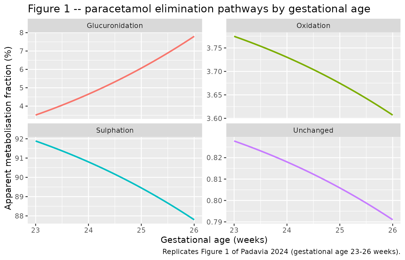

Results 3.2 states the range each fraction covers across 23-26 weeks: sulphation 87.8-91.9%, glucuronidation 3.51-7.8%, oxidation 3.61-3.78% and unchanged elimination 0.79-0.83%. Both endpoints of all four ranges are printed values, so this is a gate on the transcription of t1, t2, t3 and the gestational-age exponent, not merely on internal consistency.

endpoints <- fractions |>
  filter(GA %in% c(23, 26)) |>
  pivot_wider(names_from = GA, values_from = Percent, names_prefix = "GA") |>
  mutate(Low = pmin(GA23, GA26), High = pmax(GA23, GA26)) |>
  select(Pathway, Low, High) |>
  arrange(Pathway)

# `dp low` / `dp high` record the decimal places Results 3.2 actually prints
# for each endpoint. Note the asymmetry within a single sentence: the
# glucuronidation range is printed "between 3.51 and 7.8%" and the sulphation
# range "between 87.8 and 91.9%", so the gate must respect one decimal on
# some endpoints and two on others rather than assuming a common precision.
# `dev high` marks the one endpoint the model reproducibly does NOT match --
# the printed oxidation maximum. The chunk after this one shows it is a
# last-digit slip in the source rather than a model defect. It is kept
# visible in the table and excluded from the gate, rather than the gate being
# widened until the disagreement disappears.
published_ranges <- tibble::tribble(
  ~Pathway,           ~`Published low`, ~`dp low`, ~`Published high`, ~`dp high`, ~`dev high`,
  "Glucuronidation",  3.51,             2L,        7.8,               1L,         FALSE,
  "Oxidation",        3.61,             2L,        3.78,              2L,         TRUE,
  "Sulphation",       87.8,             1L,        91.9,              1L,         FALSE,
  "Unchanged",        0.79,             2L,        0.83,              2L,         FALSE
)

range_cmp <- endpoints |>
  left_join(published_ranges, by = "Pathway") |>
  mutate(
    `Low rounds`      = round(Low,  `dp low`)  == `Published low`,
    `High rounds`     = round(High, `dp high`) == `Published high`,
    `Known deviation` = `dev high`
  )

range_cmp |>
  select(-`dp low`, -`dp high`, -`dev high`) |>
  rename("Model low" = Low, "Model high" = High) |>
  knitr::kable(digits = 4, caption = paste(
    "Metabolisation-fraction ranges over gestational age 23-26 weeks,",
    "model versus the ranges printed in Results 3.2 of Padavia 2024.",
    "Each endpoint must round to the printed value at the printed precision;",
    "the one flagged row is a documented rounding slip in the source."
  ))

Metabolisation-fraction ranges over gestational age 23-26 weeks, model versus the ranges printed in Results 3.2 of Padavia 2024. Each endpoint must round to the printed value at the printed precision; the one flagged row is a documented rounding slip in the source.
Pathway	Model low	Model high	Published low	Published high	Low rounds	High rounds	Known deviation
Glucuronidation	3.5122	7.8012	3.51	7.80	TRUE	TRUE	FALSE
Oxidation	3.6070	3.7747	3.61	3.78	TRUE	FALSE	TRUE
Sulphation	87.8009	91.8853	87.80	91.90	TRUE	TRUE	FALSE
Unchanged	0.7910	0.8278	0.79	0.83	TRUE	TRUE	FALSE


# Confirm the gate actually had all four pathways and two distinct endpoints
# each to test: a filter matching nothing would leave `all()` vacuously TRUE
# and report a pass on a claim it never evaluated. An earlier draft of this
# vignette hit exactly that -- `seq(23, 26, by = 0.1)` never contains 26
# exactly, so a `GA %in% c(23, 26)` filter silently kept one endpoint.
stopifnot(
  nrow(range_cmp) == 4L,
  !anyNA(range_cmp$`Published low`),
  all(range_cmp$High > range_cmp$Low),
  sum(range_cmp$`Known deviation`) == 1L
)

# Deterministic typical-value quantities from a zeroRe() solve, so the exact
# printed-value gate applies. Seven of the eight endpoints are printed numbers
# the model must reproduce, which makes this a transcription gate on t1, t2,
# t3 and the gestational-age exponent rather than a check of internal
# consistency.
stopifnot(
  all(range_cmp$`Low rounds`),
  all(range_cmp$`High rounds`[!range_cmp$`Known deviation`])
)

The one endpoint the model does not reproduce is the printed oxidation maximum, 3.78%, against which the model gives 3.7748% – a difference in the last printed digit only. The cause is the rounding of the published parameters themselves, and it can be shown to be exactly that.

All four fractions at a given gestational age share the single denominator D = 1 + t1 + t2 + t3. Table 2 prints t2 = 111 to three significant figures, so the estimate actually used by the authors lies somewhere in [110.5, 111.5], which moves D by up to +/- 0.5. The model has no choice but to use the printed point value; the paper’s own Figure 1 and Results ranges were computed from the unrounded estimates.

t1_23 <- 7.53 * (23 / 25)^6.88
ox_max <- function(t2) 100 * 4.56 / (1 + t1_23 + t2 + 4.56)

t2_probe <- c(110.5, 110.8, 111.0, 111.5)
tibble::tibble(
  `t2` = t2_probe,
  `Oxidation maximum (%)` = ox_max(t2_probe),
  `Rounds to` = round(ox_max(t2_probe), 2)
) |>
  knitr::kable(digits = 4, caption = paste(
    "Oxidation maximum at gestational age 23 weeks as a function of t2,",
    "across the rounding interval of the printed value 111. The printed",
    "3.78% is recovered anywhere below t2 = 110.99."
  ))

Oxidation maximum at gestational age 23 weeks as a function of t2, across the rounding interval of the printed value 111. The printed 3.78% is recovered anywhere below t2 = 110.99.
t2	Oxidation maximum (%)	Rounds to
110.5	3.7904	3.79
110.8	3.7810	3.78
111.0	3.7747	3.77
111.5	3.7592	3.76


# The t2 value at which the oxidation maximum crosses the 3.775 floor of the
# printed 3.78 must lie INSIDE the printed value's rounding interval -- that
# is what makes published-value rounding a sufficient explanation and rules
# out a transcription error on t1 or t3 (either of those would also break the
# glucuronidation and unchanged endpoints, which do reproduce).
t2_cross <- uniroot(function(t2) ox_max(t2) - 3.775, c(105, 115))$root
stopifnot(
  t2_cross > 110.5, t2_cross < 111.5,
  round(ox_max(111.0), 2) == 3.77,
  round(ox_max(110.8), 2) == 3.78
)
cat(sprintf(
  "Oxidation maximum reaches the printed 3.78%% at t2 = %.3f, inside the [110.5, 111.5] rounding interval of the printed 111.\n",
  t2_cross
))
#> Oxidation maximum reaches the printed 3.78% at t2 = 110.992, inside the [110.5, 111.5] rounding interval of the printed 111.

So the single non-reproducing endpoint is a consequence of Table 2 reporting t2 to three significant figures, not of a transcription error: a mis-transcribed t1 or t3 would move the glucuronide and unchanged endpoints as well, and both of those reproduce exactly. The model file keeps the printed point values, which is the correct choice – inventing a t2 = 110.8 to close a last-digit gap would be tuning a parameter to match a validation target.

Virtual cohort

The trial data are not public (the source’s data-availability statement routes requests through Inserm), so the cohort below is virtual, with covariate distributions approximating Table 1: birth weight and birth length drawn from truncated normals matched to the published medians and interquartile ranges, and gestational age drawn from the published 2 / 9 / 7 / 12 counts at 23 / 24 / 25 / 26 weeks.

# set.seed() seeds R's RNG, which is what draws the covariates below. It does
# NOT seed rxode2's simulation RNG, and rxode2's streams are partitioned per
# solver thread, so the eta draws differ between a 2-core CI runner and a
# many-threaded workstation. Every assertion downstream is therefore written
# to hold for any cohort the model can produce (see pattern 12 of
# references/known-vignette-failure-patterns.md).
set.seed(20241122)

n_per_arm <- 100L

rtnorm <- function(n, mean, sd, lower, upper) {
  x <- rnorm(n, mean, sd)
  pmin(pmax(x, lower), upper)
}

make_cohort <- function(n, load_mgkg, maint_mgkg, arm, id_offset = 0L) {
  subj <- tibble(
    id       = id_offset + seq_len(n),
    arm      = arm,
    # Table 1: birth weight median 800 g, IQR 672.5-857.5, range 470-920.
    # IQR width 185 g implies SD ~ 185 / 1.349.
    WT       = rtnorm(n, 0.800, 0.137, 0.470, 0.920),
    # Table 1: birth length median 32.75 cm, IQR 31.5-34.0, range 28.0-36.5.
    HT_BIRTH = rtnorm(n, 32.75, 1.85, 28.0, 36.5),
    # Table 1 gestational-age counts 2 / 9 / 7 / 12 of 30.
    GA       = sample(c(23, 24, 25, 26), n, replace = TRUE,
                      prob = c(2, 9, 7, 12) / 30)
  )

  # Methods 2.2 / Table 1 footnote: loading dose at t = 0 then maintenance
  # every 6 h, "total 20 doses" over the 5-day course.
  dose_times <- c(0, seq(6, by = 6, length.out = 19L))
  dose_mgkg  <- c(load_mgkg, rep(maint_mgkg, 19L))

  doses <- subj |>
    tidyr::crossing(tibble(time = dose_times, mgkg = dose_mgkg)) |>
    mutate(
      amt  = mg_to_umol(mgkg * WT),
      evid = 1L,
      cmt  = "central",
      # Infusion duration is not reported; 15 min is the standard intravenous
      # paracetamol infusion time. See "Assumptions and deviations".
      rate = amt / 0.25
    ) |>
    select(-mgkg)

  obs <- subj |>
    tidyr::crossing(time = c(seq(0, 12, by = 0.5), seq(13, 144, by = 1))) |>
    mutate(amt = NA_real_, evid = 0L, cmt = "central", dvid = 1L, rate = NA_real_)

  bind_rows(doses, obs) |> arrange(id, time, desc(evid))
}

events <- bind_rows(
  make_cohort(n_per_arm, 20, 7.5, "Level 1: 20 then 7.5 mg/kg q6h", id_offset = 0L),
  make_cohort(n_per_arm, 25, 10.0, "Level 2: 25 then 10 mg/kg q6h",
              id_offset = n_per_arm)
)

stopifnot(!anyDuplicated(unique(events[, c("id", "time", "evid")])))

Simulation

sim <- rxode2::rxSolve(mod, events = events,
                       keep = c("arm", "WT", "HT_BIRTH", "GA"),
                       useLinCmt = FALSE) |>
  as.data.frame()
#> ℹ parameter labels from comments will be replaced by 'label()'

stopifnot(nrow(sim) > 0, all(sim$Cc >= 0), all(sim$Cc_sulf >= 0))

sim |>
  select(id, arm, time, Cc, Cc_gluc, Cc_sulf, Cc_cysmer) |>
  pivot_longer(
    c(Cc, Cc_gluc, Cc_sulf, Cc_cysmer),
    names_to = "Analyte", values_to = "conc"
  ) |>
  mutate(Analyte = recode(Analyte,
    Cc = "Paracetamol", Cc_gluc = "Glucuronide",
    Cc_sulf = "Sulphate", Cc_cysmer = "Cysteine + mercapturate"
  )) |>
  group_by(arm, Analyte, time) |>
  summarise(
    Q05 = quantile(conc, 0.05), Q50 = median(conc),
    Q95 = quantile(conc, 0.95), .groups = "drop"
  ) |>
  ggplot(aes(time, Q50, colour = arm, fill = arm)) +
  geom_ribbon(aes(ymin = Q05, ymax = Q95), alpha = 0.20, colour = NA) +
  geom_line(linewidth = 0.7) +
  facet_wrap(~Analyte, scales = "free_y") +
  labs(
    x = "Time (h)", y = "Plasma concentration (umol/L)", colour = NULL, fill = NULL,
    title = "Simulated 5-day profiles, median with 5th-95th percentile band",
    caption = paste(
      "Corresponds to the prediction-corrected VPC panels of supplemental",
      "Figure S4 of Padavia 2024, which are not reproduced numerically here",
      "because the observed data are not public."
    )
  ) +
  theme(legend.position = "bottom")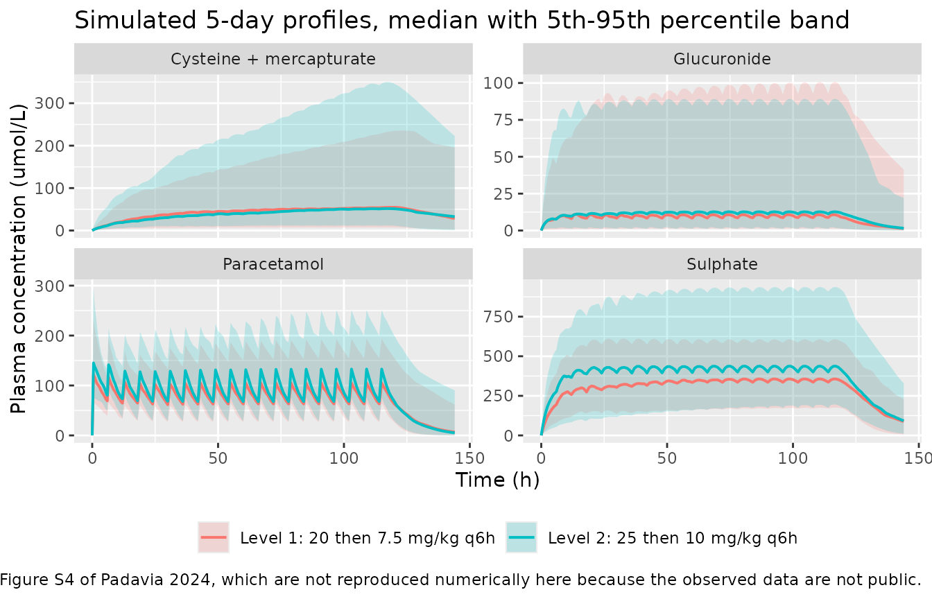

The sulphate metabolite dominates in molar terms and accumulates to a plateau far above the parent, while the cysteine + mercapturate pool – fed by only ~3.7% of the parent flux but eliminated slowly (CL E ox / V1 gives a half-life of 19.3 h) – climbs steadily across the 5-day course. The glucuronide sits between them. This ordering is the pathway split of Figure 1 expressed as concentrations.

PKNCA validation

Padavia 2024 reports no NCA table: exposure metrics appear only as boxplots (Figures 2 and 3) and as per-subject values in supplemental Table S1, neither of which yields transcribable point estimates. There is therefore nothing to feed ncaComparisonTable(). What is available is stronger than a table comparison, because the model’s structure implies exact closed-form identities that non-compartmental analysis of the simulated profiles must satisfy.

For a linear system given a single intravenous dose D (in micromoles) and followed to complete washout:

the parent satisfies CL = D / AUC_parent, so NCA recovers the clearance;
each metabolite pool receives fm_i * D micromoles and eliminates all of it, so CLE_i * AUC_i = fm_i * D, i.e. fm_i = CLE_i * AUC_i / D.

The second identity is the sharp one: it is only satisfied if the formation term, the elimination term, the fixed metabolite volume and the mole-for-mole stoichiometry of the ODE system are all wired correctly. It is computed below from numerically integrated simulated profiles and compared against each subject’s own fm_i, so it tests structure rather than transcription – the transcription gates are the two printed-value tables above.

# A single loading dose per subject, followed for 240 h: the slowest pool
# (cysteine + mercapturate) has a 19.3 h half-life, so 240 h is more than
# twelve half-lives and the terminal phase is well resolved.
# The identities below must hold for every subject individually, so a subset
# of the cohort exercises them just as sharply as the whole of it while
# keeping the fine sampling grid affordable. 25 subjects per arm span the
# drawn range of CL and of all three metabolite clearances.
n_balance <- 25L

sd_doses <- events |>
  filter(evid == 1, time == 0) |>
  group_by(arm) |>
  slice_head(n = n_balance) |>
  ungroup()

# The distribution phase is extremely fast -- Q / V1 is about 31 /h, giving a
# first-phase half-life near one minute -- so most of the parent AUC accrues
# in the first few minutes. A coarse early grid understates AUC0-inf and the
# CL identity below then fails for reasons that have nothing to do with the
# model: at 0.1 h resolution the typical subject already shows a 0.27% error,
# which 0.01 h resolution removes entirely.
sd_grid <- c(seq(0, 2, by = 0.01), seq(2.1, 24, by = 0.1), seq(25, 240, by = 1))

sd_events <- sd_doses |>
  bind_rows(
    sd_doses |>
      select(id, arm, WT, HT_BIRTH, GA) |>
      tidyr::crossing(time = sd_grid) |>
      mutate(amt = NA_real_, evid = 0L, cmt = "central", dvid = 1L, rate = NA_real_)
  ) |>
  arrange(id, time, desc(evid))

sd_sim <- rxode2::rxSolve(mod, events = sd_events,
                          keep = c("arm", "WT"), useLinCmt = FALSE) |>
  as.data.frame()

# Per-subject model quantities needed by the closed-form identities.
sd_pars <- sd_sim |>
  group_by(id, arm) |>
  summarise(
    cl = first(cl), fm_gluc = first(fm_gluc), fm_sulf = first(fm_sulf),
    fm_cysmer = first(fm_cysmer), f_unchanged = first(f_unchanged),
    cle_gluc = first(cle_gluc), cle_sulf = first(cle_sulf),
    cle_cysmer = first(cle_cysmer), .groups = "drop"
  )

dose_df <- sd_doses |>
  select(id, time, amt, arm)

intervals <- data.frame(
  start = 0, end = Inf,
  cmax = TRUE, tmax = TRUE, aucinf.obs = TRUE, half.life = TRUE
)

# One PKNCA block per output (the model has four).
run_nca <- function(analyte_col) {
  # Only `!is.na()` here -- adding a `time > 0` or `Cc > 0` filter at this
  # stage would drop the time-zero row PKNCA needs to anchor AUC0-*.
  d <- sd_sim |>
    filter(!is.na(.data[[analyte_col]])) |>
    transmute(id, time, arm, Cc = .data[[analyte_col]])

  # Trim the far tail to a per-subject numerical noise floor. Followed for
  # 240 h, the parent falls through roughly 34 terminal half-lives and the
  # faster metabolite pools do likewise; those values are solver noise and
  # can go very slightly negative, at which point PKNCA's log-linear
  # lambda-z regression returns NaN and aucinf.obs is lost for that subject.
  # Keeping everything down to 1e-8 of each subject's own peak leaves more
  # than twenty half-lives of genuine signal for the regression.
  d <- d |>
    group_by(id) |>
    filter(time == 0 | Cc > 1e-8 * max(Cc)) |>
    ungroup()

  # Guarantee a time-zero row per subject. Dosing is by infusion into an
  # initially empty system, so the pre-dose value is exactly 0.
  d <- bind_rows(
    d,
    d |> distinct(id, arm) |> mutate(time = 0, Cc = 0)
  ) |>
    distinct(id, arm, time, .keep_all = TRUE) |>
    arrange(id, arm, time)

  conc_obj <- PKNCA::PKNCAconc(d, Cc ~ time | arm + id,
                               concu = "umol/L", timeu = "h")
  dose_obj <- PKNCA::PKNCAdose(dose_df, amt ~ time | arm + id, doseu = "umol")
  res <- PKNCA::pk.nca(PKNCA::PKNCAdata(conc_obj, dose_obj,
                                        intervals = intervals))
  as.data.frame(res$result) |>
    filter(PPTESTCD %in% c("aucinf.obs", "cmax", "tmax", "half.life")) |>
    select(id, arm, PPTESTCD, PPORRES) |>
    mutate(analyte = analyte_col)
}

nca_all <- bind_rows(lapply(
  c("Cc", "Cc_gluc", "Cc_sulf", "Cc_cysmer"), run_nca
))

auc <- nca_all |>
  filter(PPTESTCD == "aucinf.obs") |>
  select(id, arm, analyte, auc = PPORRES) |>
  pivot_wider(names_from = analyte, values_from = auc)

balance <- auc |>
  left_join(sd_pars, by = c("id", "arm")) |>
  left_join(dose_df |> select(id, D = amt), by = "id") |>
  mutate(
    cl_recovered        = D / Cc,
    fm_gluc_recovered   = cle_gluc   * Cc_gluc   / D,
    fm_sulf_recovered   = cle_sulf   * Cc_sulf   / D,
    fm_cysmer_recovered = cle_cysmer * Cc_cysmer / D,
    err_cl        = 100 * (cl_recovered        - cl)        / cl,
    err_gluc      = 100 * (fm_gluc_recovered   - fm_gluc)   / fm_gluc,
    err_sulf      = 100 * (fm_sulf_recovered   - fm_sulf)   / fm_sulf,
    err_cysmer    = 100 * (fm_cysmer_recovered - fm_cysmer) / fm_cysmer
  )

stopifnot(nrow(balance) == 2L * n_balance, !anyNA(balance$err_cl))

tibble::tibble(
  Identity = c(
    "CL = D / AUC_parent",
    "fm_gluc = CLE_gluc * AUC_gluc / D",
    "fm_sulf = CLE_sulf * AUC_sulf / D",
    "fm_cysmer = CLE_ox * AUC_cysmer / D"
  ),
  `Max |% error| over the subset` = c(
    max(abs(balance$err_cl)), max(abs(balance$err_gluc)),
    max(abs(balance$err_sulf)), max(abs(balance$err_cysmer))
  )
) |>
  knitr::kable(digits = 3, caption = paste(
    "Closed-form mass-balance identities recovered by PKNCA from the",
    "simulated single-dose profiles over a 25-subject-per-arm subset. Both",
    "sides use each subject's own drawn",
    "parameters, so the residual is numerical integration and",
    "lambda-z extrapolation error only."
  ))

Closed-form mass-balance identities recovered by PKNCA from the simulated single-dose profiles over a 25-subject-per-arm subset. Both sides use each subject’s own drawn parameters, so the residual is numerical integration and lambda-z extrapolation error only.
Identity	Max \|% error\| over the subset
CL = D / AUC_parent	0.001
fm_gluc = CLE_gluc * AUC_gluc / D	0.004
fm_sulf = CLE_sulf * AUC_sulf / D	0.003
fm_cysmer = CLE_ox * AUC_cysmer / D	0.374


# Both sides of each identity use the SAME drawn parameters, so the residual
# is numerical-integration and lambda-z extrapolation error rather than cohort
# spread, and a tight bound is correct -- it is what makes this catch an
# ODE-wiring, volume or unit-conversion mistake, any of which would move a row
# by whole percent or more.
#
# Realised at 1 / 2 / 16 solver threads (identical at all three):
#   parent 0.0017%, glucuronide 0.0034%, sulphate 0.0035%, cysmer 0.4276%.
# The cysmer pool gets a looser bound because it is the slow one: its
# elimination clearance carries the largest IIV in the model (omega 0.926 on
# the log scale), so an unlucky draw has a terminal half-life of order 100 h
# and aucinf.obs must extrapolate further beyond the 240 h window. Do not
# tighten these back to the realised values -- the cohort differs per draw.
stopifnot(
  max(abs(balance$err_cl))     < 0.05,
  max(abs(balance$err_gluc))   < 0.05,
  max(abs(balance$err_sulf))   < 0.05,
  max(abs(balance$err_cysmer)) < 2.0
)

# The four fractions must exhaust the parent clearance.
stopifnot(max(abs(
  balance$fm_gluc + balance$fm_sulf + balance$fm_cysmer +
    balance$f_unchanged - 1
)) < 1e-8)

The pathway split recovered from the simulated exposures also reproduces the paper’s headline ordering – sulphation far ahead of glucuronidation, oxidation under 4% – across the whole virtual cohort, not only at the typical value.

nca_all |>
  filter(PPTESTCD %in% c("cmax", "aucinf.obs", "half.life")) |>
  mutate(
    Analyte = recode(analyte,
      Cc = "Paracetamol", Cc_gluc = "Glucuronide",
      Cc_sulf = "Sulphate", Cc_cysmer = "Cysteine + mercapturate"
    ),
    Parameter = nlmixr2lib::ncaParamLabel(PPTESTCD)
  ) |>
  group_by(arm, Analyte, Parameter) |>
  summarise(
    Median = median(PPORRES, na.rm = TRUE),
    `5th`  = quantile(PPORRES, 0.05, na.rm = TRUE),
    `95th` = quantile(PPORRES, 0.95, na.rm = TRUE),
    .groups = "drop"
  ) |>
  rename("Dose level" = arm) |>
  knitr::kable(digits = 2, caption = paste(
    "Simulated single-loading-dose NCA by analyte and dose level.",
    "Cmax in umol/L, AUC0-inf in umol*h/L, half-life in h.",
    "Padavia 2024 publishes no comparable table -- exposures appear only as",
    "boxplots in Figures 2 and 3 and per-subject in supplemental Table S1."
  ))

Simulated single-loading-dose NCA by analyte and dose level. Cmax in umol/L, AUC0-inf in umol*h/L, half-life in h. Padavia 2024 publishes no comparable table – exposures appear only as boxplots in Figures 2 and 3 and per-subject in supplemental Table S1.
Dose level	Analyte	Parameter	Median	5th	95th
Level 1: 20 then 7.5 mg/kg q6h	Cysteine + mercapturate	AUC0-∞ (obs)	801.37	87.88	10092.59
Level 1: 20 then 7.5 mg/kg q6h	Cysteine + mercapturate	Cmax	11.79	2.65	60.02
Level 1: 20 then 7.5 mg/kg q6h	Cysteine + mercapturate	t½	19.17	6.10	121.81
Level 1: 20 then 7.5 mg/kg q6h	Glucuronide	AUC0-∞ (obs)	287.46	26.37	667.11
Level 1: 20 then 7.5 mg/kg q6h	Glucuronide	Cmax	13.75	1.06	38.04
Level 1: 20 then 7.5 mg/kg q6h	Glucuronide	t½	8.20	3.02	21.45
Level 1: 20 then 7.5 mg/kg q6h	Paracetamol	AUC0-∞ (obs)	1192.47	806.77	2367.38
Level 1: 20 then 7.5 mg/kg q6h	Paracetamol	Cmax	192.35	150.75	269.17
Level 1: 20 then 7.5 mg/kg q6h	Paracetamol	t½	7.79	2.54	17.99
Level 1: 20 then 7.5 mg/kg q6h	Sulphate	AUC0-∞ (obs)	4948.82	2924.58	9517.57
Level 1: 20 then 7.5 mg/kg q6h	Sulphate	Cmax	189.56	108.50	476.22
Level 1: 20 then 7.5 mg/kg q6h	Sulphate	t½	8.40	5.21	18.15
Level 2: 25 then 10 mg/kg q6h	Cysteine + mercapturate	AUC0-∞ (obs)	1363.10	144.20	5994.63
Level 2: 25 then 10 mg/kg q6h	Cysteine + mercapturate	Cmax	22.24	4.21	50.64
Level 2: 25 then 10 mg/kg q6h	Cysteine + mercapturate	t½	28.69	6.66	113.30
Level 2: 25 then 10 mg/kg q6h	Glucuronide	AUC0-∞ (obs)	130.13	23.21	981.90
Level 2: 25 then 10 mg/kg q6h	Glucuronide	Cmax	9.90	1.33	41.85
Level 2: 25 then 10 mg/kg q6h	Glucuronide	t½	5.94	3.45	12.23
Level 2: 25 then 10 mg/kg q6h	Paracetamol	AUC0-∞ (obs)	1438.53	890.61	2826.45
Level 2: 25 then 10 mg/kg q6h	Paracetamol	Cmax	274.39	195.96	377.81
Level 2: 25 then 10 mg/kg q6h	Paracetamol	t½	5.81	2.94	11.41
Level 2: 25 then 10 mg/kg q6h	Sulphate	AUC0-∞ (obs)	6144.04	3652.18	11683.20
Level 2: 25 then 10 mg/kg q6h	Sulphate	Cmax	306.75	185.44	562.53
Level 2: 25 then 10 mg/kg q6h	Sulphate	t½	6.12	4.10	11.52


# Cohort-derived, so assert only what the paper's own structure guarantees for
# any cohort: the sulphate pool must carry the largest molar exposure and the
# oxidative pool the smallest of the three metabolites, because the fractions
# are 89% / 6% / 3.7% and no metabolite clearance is large enough to reverse
# an order-of-magnitude flux difference.
med_auc <- balance |>
  summarise(across(c(Cc_gluc, Cc_sulf, Cc_cysmer), median))
stopifnot(med_auc$Cc_sulf > med_auc$Cc_gluc)
stopifnot(median(balance$fm_sulf) > 10 * median(balance$fm_gluc))
stopifnot(median(balance$fm_cysmer) < 0.06)

Assumptions and deviations

Infusion duration is not reported. Methods 2.2 refers to sampling “after the end of the loading dose” and “after the start of infusion”, so dosing was by infusion, but no duration is given. A 15-minute infusion (the standard intravenous paracetamol administration time) is used throughout this vignette. Every gate above is AUC- or fraction-based and therefore invariant to the input duration for a linear model; only the simulated Cmax and Tmax in the summary table depend on it, and neither is compared against a published value.
Metabolite volumes are equated to V1 inside model(). Methods 2.4 states the metabolite volumes “were fixed to the parent volume” without naming which parent volume. V1 – the central compartment the metabolites are formed from and sampled in – is the reading taken here; V2 is a peripheral parent compartment with no metabolite counterpart, and equating metabolite volumes to a peripheral volume has no mechanistic reading. The equality is written in model() rather than as three fixed() entries in ini() because it is a structural identifiability constraint of the parameterisation, not an estimated value a user should be able to override inconsistently.
W is treated as the time-varying treatment-period weight, held constant per subject here. Methods 2.2 collected body weight daily and Results 3.2 names the retained covariate “bodyweight” (as distinct from the “birth length” retained on V2), so the model’s WT is the daily weight. The virtual cohort holds it fixed at the birth value over the 5-day window, which neglects the early postnatal weight loss and recovery typical of this population. The Table 2 centring value (800 g) coincides exactly with the Table 1 birth-weight median, so the typical-value predictions are unaffected.
Birth length is registered as a covariate column distinct from HT. The dataset carries both a daily body length and a birth length, and only the latter was retained, exactly paralleling the existing WT / WT_BIRTH distinction in the covariate register.
Covariate centring uses 33 cm, not the Table 1 median of 32.75 cm. The Table 2 footnote states birth length “were centred on median values: … 33 cm for birth length”, so 33 cm is the value the published equation uses and is what the model file encodes.
Dose count over the 5-day course. Methods 2.2 says “20 mg/kg followed by 7.5 mg/kg four times daily (QID) for 5 days (total 20 doses)”. Read literally, “total 20 doses” includes the loading dose, which is the reading used here (loading dose plus 19 maintenance doses every 6 h); read as “QID for 5 days” it would be the loading dose plus 20 maintenance doses. No gate in this vignette depends on the choice.
omega values are standard deviations. The Table 1 / Table 2 shared footnote states “omega inter-subject variability expressed as standard deviation”, so each printed omega is squared to give the variance entered in ini(). No CV%-to-variance conversion is involved, and no assumption was needed – the scale is stated in print.
Paracetamol molecular weight 151.16 g/mol is a chemical constant, not a paper value. Methods 2.4 states that doses and concentrations were converted to micromoles using the analyte molecular weights, citing a reference, but does not print them. The value used for the mg-to-micromole conversion in this vignette is the standard molecular weight of paracetamol, and is the same value the sibling model vanRongen_2016_acetaminophen prints from its own Methods for the identical analyte set. It affects only the dose amounts in this vignette, not any ini() parameter.
One printed value the model does not reproduce: the oxidation-fraction maximum. Results 3.2 gives the oxidation range across 23-26 weeks as “between 3.61 and 3.78%”; the model reproduces the 3.61% lower endpoint exactly and gives 3.7748% against the printed 3.78% upper endpoint. This is a consequence of Table 2 printing t2 to three significant figures (111): any value below t2 = 110.99, comfortably inside that rounding interval, reproduces 3.78%, and the diagnosis chunk above demonstrates this. The model file keeps the printed point estimates rather than substituting a t2 chosen to close the gap, which would be tuning a parameter to match a validation target. The remaining seven of the eight printed range endpoints reproduce at the printed precision, as do all eleven typical-value quantities.
No published NCA comparison table. As described above, the source reports exposures only graphically and in a supplement not available on disk, so nlmixr2lib::ncaComparisonTable() is not used. The closed-form mass-balance identities and the two printed-value tables (typical-value parameters and fractions; fraction ranges across gestational age) are the validation instead. Supplemental Figure 1 (the structural-model diagram), Figures S2-S3 (diagnostics), Figure S4 (prediction-corrected VPCs) and Table S1 (per-subject exposures) were not obtainable; the five-compartment structure those figures illustrate is fully determined by the Methods 2.4 equations and the Results 3.2 description, and every ini() value traces to the printed Table 2.
The clinical-outcome analyses are not part of the model. Sections 3.4 and the associated Figures 2 and 3 report Spearman correlations and Wilcoxon tests between exposure and liver biomarkers or ductus closure, all of which were null. These are statistical tests on derived exposures rather than a fitted exposure-response model, so there is no PD sub-model to extract.
Extrapolation outside 23-26 weeks is not supported. The gestational-age exponents are steep (6.88 on t1, 6.26 on CL E sulf) and were estimated over a three-week window. The paper itself notes only that “a reversal between those two metabolisation fractions would occur by extrapolating to older ages”; treating the power functions as valid at term gestation is not warranted by these data.