Model and source
- Citation: Offman E, Singh N, Julian MW, Locke LW, Bicer S, Mitchell J, Matthews T, Anderson K, Crouser ED. Leveraging in vitro and pharmacokinetic models to support bench to bedside investigation of XTMAB-16 as a novel pulmonary sarcoidosis treatment. Front Pharmacol. 2023;14:1066454. doi:10.3389/fphar.2023.1066454. Final parameter estimates from Supplementary Table S4; structural and covariate model from the Results section ‘Model development and qualification’.
- Description: Two-compartment population PK model with linear elimination for XTMAB-16, a chimeric anti-TNF-alpha monoclonal antibody, after a single 2-h intravenous infusion of 2 or 4 mg/kg in 19 healthy adults of the first-in-human study XTMAB-16-101 (NCT04971395; Offman 2023 Supplementary Table S4). Central and peripheral volumes share one estimated body-weight power exponent (reference 72.4 kg); clearance is multiplied by 1.274 in subjects who were ever anti-drug-antibody positive. IIV on CL, V and V2; combined additive plus proportional residual error.
- Article: https://doi.org/10.3389/fphar.2023.1066454
- Supplement (Supplementary Methods and Tables S1-S7): https://www.frontiersin.org/articles/10.3389/fphar.2023.1066454/full#supplementary-material
XTMAB-16 is a chimeric anti-TNF-alpha monoclonal antibody in development for pulmonary sarcoidosis. Offman 2023 combines an in vitro granuloma assay (peripheral blood mononuclear cells from patients with sarcoidosis) with a population PK model fitted to the first-in-human study, and uses simulations from that model to propose 2 and 4 mg/kg doses every 2 or 4 weeks. This package contains the population PK model.
Population
The PK model was fitted in Phoenix NLME 8.4 to 277 serum samples (226 quantifiable) from the 19 healthy adults who received XTMAB-16 as a single 2-hour intravenous infusion of 2 mg/kg (n = 10) or 4 mg/kg (n = 9) in the randomised, double-blind, placebo-controlled study XTMAB-16-101 (NCT04971395). Per Table 1, body weight was 53.2-97.2 kg (median 72.4 kg), age 19-45 years (median 32 years), 68.4% were female, 84.2% Black or African American, 10.5% White and 5.3% American Indian or Alaska Native, and 8 of 19 subjects (42.1%) had at least one ADA-positive sample. All of them also had neutralising ADA. Samples below the limit of quantitation were set to missing.
The same information is available programmatically via
readModelDb("Offman_2023_XTMAB16")()$population.
Source trace
Every ini() value carries an in-file comment pointing to
Supplementary Table S4 of Offman 2023. The table below collects
them.
| Equation / parameter | Value | Source location |
|---|---|---|
lcl (CL, ADA-negative) |
log(0.00902 L/h) | Table S4, CL row |
e_ada_pos_cl |
1.274 | Table S4, CL row: “x 1.274 if subject is ADA positive” |
lvc (V at 72.4 kg) |
log(2.30 L) | Table S4, V row |
lvp (V2 at 72.4 kg) |
log(0.715 L) | Table S4, V2 row |
e_wt_vc (shared by V and V2) |
0.426 | Table S4, V and V2 rows: (Weight/72.4)^0.426 |
lq |
log(0.0119 L/h) | Table S4, Q row |
etalcl |
0.0246 (variance) | Table S4, IIV on CL; footnote a: variances |
etalvc |
0.00936 (variance) | Table S4, IIV on V |
etalvp |
0.203 (variance) | Table S4, IIV on V2 |
propSd |
0.0689 | Table S4, proportional error 6.89% |
addSd |
0.819 mg/L | Table S4, additive error 819 ng/mL |
| Two-compartment model, linear elimination, IIV on CL, V and V2 only (none on Q) | n/a | Results, “Model development and qualification” |
| Combined additive + proportional residual error | n/a | Results, “Model development and qualification” |
Clung = 0.149 * Cc (vignette only) |
0.149 | Methods, “Simulations”: antibody biodistribution coefficient for lung (14.9%, Li et al. 2016) |
Typical-value checks
The paper reports derived quantities for a typical subject in the Results text (CL 0.009 L/h, Vss 3.02 L and a half-life of 243.3 h at 72.4 kg, 194.0 h if ADA-positive). These follow in closed form from the model parameters, so they are checked to rounding precision.
mod <- readModelDb("Offman_2023_XTMAB16")
th <- rxode2::rxode(mod)$theta
#> ℹ parameter labels from comments will be replaced by 'label()'

terminal_half_life <- function(cl, vc, vp, q) {
  k10 <- cl / vc
  k12 <- q / vc
  k21 <- q / vp
  a <- k10 + k12 + k21
  lambda_z <- (a - sqrt(a^2 - 4 * k10 * k21)) / 2
  log(2) / lambda_z
}

cl_neg <- exp(th[["lcl"]])
vc_ref <- exp(th[["lvc"]])
vp_ref <- exp(th[["lvp"]])
q_ref <- exp(th[["lq"]])

typical <- tibble::tribble(
  ~quantity, ~paper, ~model,
  "Vss at 72.4 kg (L)", 3.02, vc_ref + vp_ref,
  "t1/2, ADA-negative (h)", 243.3, terminal_half_life(cl_neg, vc_ref, vp_ref, q_ref),
  "t1/2, ADA-positive (h)", 194.0,
  terminal_half_life(cl_neg * th[["e_ada_pos_cl"]], vc_ref, vp_ref, q_ref)
) |>
  mutate(pct_diff = 100 * (model - paper) / paper)

typical |>
  dplyr::rename(
    "Quantity" = quantity,
    "Offman 2023" = paper,
    "Model" = model,
    "% diff" = pct_diff
  ) |>
knitr::kable(digits = 2, caption = "Closed-form typical-value quantities vs. the Offman 2023 Results text.")| Quantity | Offman 2023 | Model | % diff |
|---|---|---|---|
| Vss at 72.4 kg (L) | 3.02 | 3.01 | -0.17 |
| t1/2, ADA-negative (h) | 243.30 | 243.05 | -0.10 |
| t1/2, ADA-positive (h) | 194.00 | 193.67 | -0.17 |
Single-dose NCA (Supplementary Table S7)
Supplementary Table S7 lists NCA parameters from the authors’ simulation of a typical 70 kg ADA-negative subject after one 2-h infusion. The Q4W rows use a 672-h (4-week) window and are compared here; the Q2W rows differ only by the shorter 336-h window and give the 336-h trough.
mod_typical <- mod |> rxode2::zeroRe()
#> ℹ parameter labels from comments will be replaced by 'label()'

make_single_dose <- function(id, mgkg, wt = 70, end = 672) {
  amt <- mgkg * wt
  dose <- data.frame(
    id = id, time = 0, amt = amt, rate = amt / 2, evid = 1, cmt = "central"
  )
  obs <- data.frame(
    id = id, time = sort(unique(c(seq(0, 4, by = 0.25), seq(6, end, by = 2)))),
    amt = 0, rate = 0, evid = 0, cmt = "central"
  )
  dplyr::bind_rows(dose, obs) |>
    dplyr::mutate(WT = wt, ADA_POS = 0, treatment = paste(mgkg, "mg/kg")) |>
    dplyr::arrange(id, time, dplyr::desc(evid))
}

events_sd <- dplyr::bind_rows(make_single_dose(1L, 2), make_single_dose(2L, 4))
sim_sd <- rxode2::rxSolve(mod_typical, events = events_sd, keep = "treatment") |>
  as.data.frame()
#> ℹ omega/sigma items treated as zero: 'etalcl', 'etalvc', 'etalvp'
#> Warning: multi-subject simulation without without 'omega'
sim_nca <- sim_sd |>
  dplyr::filter(!is.na(Cc)) |>
  dplyr::select(id, time, Cc, treatment)
# The infusion starts at time 0, so the pre-dose concentration is 0.
stopifnot(all(sim_nca$Cc[sim_nca$time == 0] == 0))

conc_obj <- PKNCA::PKNCAconc(sim_nca, Cc ~ time | treatment + id)
dose_df <- events_sd |>
  dplyr::filter(evid == 1) |>
  dplyr::mutate(duration = amt / rate) |>
  dplyr::select(id, time, amt, duration, treatment)
dose_obj <- PKNCA::PKNCAdose(
  dose_df, amt ~ time | treatment + id,
  route = "intravascular", duration = "duration"
)
intervals <- data.frame(
  start = 0, end = Inf,
  cmax = TRUE, tmax = TRUE, aucinf.obs = TRUE, half.life = TRUE,
  mrt.iv.obs = TRUE, vss.iv.obs = TRUE, vz.obs = TRUE, cl.obs = TRUE
)
nca_res <- PKNCA::pk.nca(PKNCA::PKNCAdata(conc_obj, dose_obj, intervals = intervals))

# Table S7, Q4W rows (2 and 4 mg/kg). Vz, Vss and CL are printed per kg and
# are converted to a 70 kg subject (mL/kg x 70 / 1000 = L).
published <- tibble::tribble(
  ~treatment, ~cmax, ~tmax, ~aucinf.obs, ~half.life, ~mrt.iv.obs, ~vz.obs, ~vss.iv.obs, ~cl.obs,
  "2 mg/kg", 61.1, 2, 15500, 238, 329, 44.2 * 70 / 1000, 42.4 * 70 / 1000, 0.129 * 70 / 1000,
  "4 mg/kg", 122, 2, 31000, 238, 329, 44.2 * 70 / 1000, 42.4 * 70 / 1000, 0.129 * 70 / 1000
)

cmp <- nlmixr2lib::ncaComparisonTable(
  simulated = nca_res,
  reference = published,
  by = "treatment",
  units = c(
    cmax = "ug/mL", tmax = "h", aucinf.obs = "h*ug/mL", half.life = "h",
    mrt.iv.obs = "h", vz.obs = "L", vss.iv.obs = "L", cl.obs = "L/h"
  ),
  tolerance_pct = 20
)
knitr::kable(
  cmp,
  caption = "Typical 70 kg ADA-negative subject, single 2-h infusion: PKNCA on the packaged model vs. Offman 2023 Supplementary Table S7 (Q4W rows). * differs from reference by >20%."
)| NCA parameter | treatment | Reference | Simulated | % diff |
|---|---|---|---|---|
| Cmax (ug/mL) | 2 mg/kg | 61.1 | 61.2 | +0.1% |
| Cmax (ug/mL) | 4 mg/kg | 122 | 122 | +0.3% |
| Tmax (h) | 2 mg/kg | 2 | 2 | +0.0% |
| Tmax (h) | 4 mg/kg | 2 | 2 | +0.0% |
| AUC0-∞ (obs) (h*ug/mL) | 2 mg/kg | 15500 | 15500 | +0.0% |
| AUC0-∞ (obs) (h*ug/mL) | 4 mg/kg | 31000 | 31000 | +0.0% |
| t½ (h) | 2 mg/kg | 238 | 237 | -0.2% |
| t½ (h) | 4 mg/kg | 238 | 237 | -0.2% |
| CL/F (L/h) | 2 mg/kg | 0.00903 | 0.00903 | +0.0% |
| CL/F (L/h) | 4 mg/kg | 0.00903 | 0.00903 | +0.0% |
| MRT (IV) (h) | 2 mg/kg | 329 | 328 | -0.2% |
| MRT (IV) (h) | 4 mg/kg | 329 | 328 | -0.2% |
| Vss (IV) (L) | 2 mg/kg | 2.97 | 2.96 | -0.1% |
| Vss (IV) (L) | 4 mg/kg | 2.97 | 2.96 | -0.1% |
| Vz/F (L) | 2 mg/kg | 3.09 | 3.09 | +0.0% |
| Vz/F (L) | 4 mg/kg | 3.09 | 3.09 | +0.0% |
# Deterministic typical-value simulation compared with the authors' own
# typical-value simulation: differences come only from the NCA time grid
# and terminal-phase point selection.
pct <- as.numeric(gsub("[^0-9.-]", "", as.character(cmp[["% diff"]])))
stopifnot(length(pct) == 16, !anyNA(pct), all(abs(pct) < 5))

trough_336 <- sim_sd |>
  dplyr::filter(time == 336) |>
  dplyr::select(treatment, Cc)
trough_336
#>   treatment       Cc
#> 1   2 mg/kg 16.13452
#> 2   4 mg/kg 32.26903
# Table S7 Q2W rows: Ctrough at 336 h = 16.1 and 32.3 ug/mL.
stopifnot(all(abs(trough_336$Cc / c(16.1, 32.3) - 1) < 0.02))
Repeated-dose exposure (Supplementary Tables S5 and S6)
The authors simulated six doses Q2W or three doses Q4W over the first 12 weeks and report, for a typical 70 kg ADA-negative subject, the trough after the first dosing interval, the trough at the end of the last interval (week 12), and the average concentration over that last interval. Lung interstitial concentrations (Table S6) are the serum concentrations multiplied by the antibody biodistribution coefficient of 14.9% for lung (Methods, “Simulations”).
abc_lung <- 0.149

make_regimen <- function(id, mgkg, tau, n_dose, wt = 70, ada_pos = 0, grid = 1) {
  amt <- mgkg * wt
  dose <- data.frame(
    id = id, time = (seq_len(n_dose) - 1) * tau, amt = amt, rate = amt / 2,
    evid = 1, cmt = "central"
  )
  obs <- data.frame(
    id = id, time = seq(0, 16 * 168, by = grid),
    amt = 0, rate = 0, evid = 0, cmt = "central"
  )
  dplyr::bind_rows(dose, obs) |>
    dplyr::mutate(
      WT = wt, ADA_POS = ada_pos,
      regimen = paste(mgkg, "mg/kg", ifelse(tau == 336, "Q2W", "Q4W")),
      tau = tau
    ) |>
    dplyr::arrange(id, time, dplyr::desc(evid))
}

events_md <- dplyr::bind_rows(
  make_regimen(1L, 2, 336, 6),
  make_regimen(2L, 4, 336, 6),
  make_regimen(3L, 2, 672, 3),
  make_regimen(4L, 4, 672, 3)
)
sim_md <- rxode2::rxSolve(mod_typical, events = events_md, keep = c("regimen", "tau")) |>
  as.data.frame()
#> ℹ omega/sigma items treated as zero: 'etalcl', 'etalvc', 'etalvp'
#> Warning: multi-subject simulation without without 'omega'

week12 <- 12 * 168
md_summary <- sim_md |>
  dplyr::group_by(regimen) |>
  dplyr::summarise(
    ctrough_first = Cc[time == tau[1]],
    ctrough_last = Cc[time == week12],
    cavg_last = {
      keep_rows <- time >= week12 - tau[1] & time <= week12
      tt <- time[keep_rows]
      cc <- Cc[keep_rows]
      sum(diff(tt) * (head(cc, -1) + tail(cc, -1)) / 2) / tau[1]
    },
    .groups = "drop"
  )

published_md <- tibble::tribble(
  ~regimen, ~pub_ctrough_first, ~pub_ctrough_last, ~pub_cavg_last, ~pub_lung_ctrough_first, ~pub_lung_ctrough_last,
  "2 mg/kg Q2W", 16.1, 25.9, 46.1, 2.40, 3.86,
  "4 mg/kg Q2W", 32.3, 51.8, 92.1, 4.81, 7.71,
  "2 mg/kg Q4W", 6.11, 7.11, 23.0, 0.91, 1.06,
  "4 mg/kg Q4W", 12.2, 14.2, 46.1, 1.82, 2.12
)

md_cmp <- md_summary |>
  dplyr::left_join(published_md, by = "regimen") |>
  dplyr::mutate(
    lung_ctrough_first = abc_lung * ctrough_first,
    lung_ctrough_last = abc_lung * ctrough_last
  )

md_cmp |>
  dplyr::select(
    regimen, ctrough_first, pub_ctrough_first, ctrough_last, pub_ctrough_last,
    cavg_last, pub_cavg_last, lung_ctrough_last, pub_lung_ctrough_last
  ) |>
  dplyr::rename(
    "Regimen" = regimen,
    "Serum Ctrough 1st interval, model" = ctrough_first,
    "Serum Ctrough 1st interval, Table S5" = pub_ctrough_first,
    "Serum Ctrough week 12, model" = ctrough_last,
    "Serum Ctrough week 12, Table S5" = pub_ctrough_last,
    "Serum Cavg last interval, model" = cavg_last,
    "Serum Cavg last interval, Table S5" = pub_cavg_last,
    "Lung Ctrough week 12, model" = lung_ctrough_last,
    "Lung Ctrough week 12, Table S6" = pub_lung_ctrough_last
  ) |>
  knitr::kable(
    digits = 2,
    caption = "Typical 70 kg ADA-negative subject (ug/mL): packaged model vs. Offman 2023 Supplementary Tables S5 (serum) and S6 (lung)."
)| Regimen | Serum Ctrough 1st interval, model | Serum Ctrough 1st interval, Table S5 | Serum Ctrough week 12, model | Serum Ctrough week 12, Table S5 | Serum Cavg last interval, model | Serum Cavg last interval, Table S5 | Lung Ctrough week 12, model | Lung Ctrough week 12, Table S6 |
|---|---|---|---|---|---|---|---|---|
| 2 mg/kg Q2W | 16.13 | 16.10 | 25.87 | 25.90 | 46.07 | 46.1 | 3.85 | 3.86 |
| 2 mg/kg Q4W | 6.10 | 6.11 | 7.10 | 7.11 | 23.03 | 23.0 | 1.06 | 1.06 |
| 4 mg/kg Q2W | 32.27 | 32.30 | 51.74 | 51.80 | 92.13 | 92.1 | 7.71 | 7.71 |
| 4 mg/kg Q4W | 12.20 | 12.20 | 14.20 | 14.20 | 46.07 | 46.1 | 2.12 | 2.12 |
ratio <- with(md_cmp, c(
  ctrough_first / pub_ctrough_first, ctrough_last / pub_ctrough_last,
  cavg_last / pub_cavg_last, lung_ctrough_first / pub_lung_ctrough_first,
  lung_ctrough_last / pub_lung_ctrough_last
))
# Typical-value solve against the authors' typical-value simulation;
# printed to three significant figures.
stopifnot(all(abs(ratio - 1) < 0.02))
Concentration-time profiles by dose (Figure 4)
Figure 4 of Offman 2023 shows the observed mean (+SD) serum concentrations after a single 2 or 4 mg/kg infusion. A virtual cohort of 200 subjects per dose with body weight drawn from the study distribution (Table 1: mean 72.3 kg, SD 11.7 kg, range 53.2-97.2 kg) and 42.1% subject-level ADA positivity is simulated over the study sampling schedule (days 1-8, 15, 29, 43, 57 and 71; Supplementary Methods).
rxode2::rxSetSeed(20230323)
n_per_dose <- 200

make_study_cohort <- function(n, mgkg, id_offset) {
  wt <- pmin(pmax(rnorm(n, 72.3, 11.7), 53.2), 97.2)
  ada <- rbinom(n, 1, 8 / 19)
  obs_times <- sort(unique(c(
    0, 1, 2, 4, 8, 12, 24 * (1:7), 24 * c(14, 28, 42, 56, 70)
  )))
  subjects <- lapply(seq_len(n), function(i) {
    amt <- mgkg * wt[i]
    dplyr::bind_rows(
      data.frame(time = 0, amt = amt, rate = amt / 2, evid = 1),
      data.frame(time = obs_times, amt = 0, rate = 0, evid = 0)
    ) |>
      dplyr::mutate(id = id_offset + i, WT = wt[i], ADA_POS = ada[i])
  })
  dplyr::bind_rows(subjects) |>
    dplyr::mutate(cmt = "central", treatment = paste(mgkg, "mg/kg")) |>
    dplyr::arrange(id, time, dplyr::desc(evid))
}

events_fig4 <- dplyr::bind_rows(
  make_study_cohort(n_per_dose, 2, 0L),
  make_study_cohort(n_per_dose, 4, n_per_dose)
)
stopifnot(!anyDuplicated(unique(events_fig4[, c("id", "time", "evid")])))

sim_fig4 <- rxode2::rxSolve(mod, events = events_fig4, keep = "treatment") |>
  as.data.frame()
#> ℹ parameter labels from comments will be replaced by 'label()'

fig4 <- sim_fig4 |>
  dplyr::filter(time > 0) |>
  dplyr::mutate(conc_ngml = 1000 * Cc) |>
  dplyr::group_by(treatment, time) |>
  dplyr::summarise(
    mean = mean(conc_ngml), sd = stats::sd(conc_ngml),
    .groups = "drop"
  )

ggplot(fig4, aes(time, mean, colour = treatment)) +
  geom_line() +
  geom_point() +
  geom_errorbar(aes(ymin = mean, ymax = mean + sd), width = 15) +
  scale_y_log10() +
  scale_x_continuous(breaks = seq(0, 1680, by = 336)) +
  labs(
    x = "Nominal time (h)", y = "Mean (+SD) XTMAB-16 concentration (ng/mL)",
    colour = NULL,
    title = "Single-dose serum concentrations by dose",
    caption = "Replicates Figure 4B of Offman 2023 (semi-log panel)."
  ) +
  theme_bw() +
  theme(legend.position = "bottom")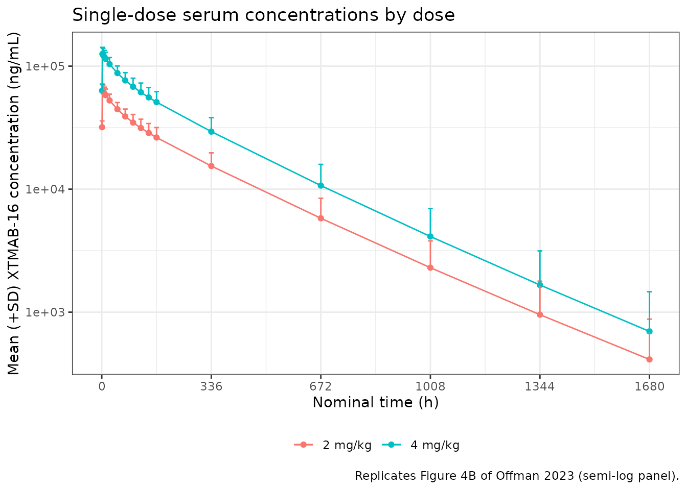
The simulated means can be read against Figure 4B: about 60,000 and 120,000 ng/mL at the end of infusion, falling to roughly 25,000 and 55,000 ng/mL at 168 h. From 1008 h on the observed means in Figure 4B (about 4,600 ng/mL at 1008 h for both doses) lie above the simulated ones; the figure note states that BLQ samples after Tmax were set to missing before averaging, so the late observed means are over the quantifiable samples only and are biased upwards, with the lower-dose arm affected most.
Lung exposure by regimen (Figure 5)
Figure 5 shows the 2.5th, 50th and 97.5th percentiles of the simulated lung concentration for 500 virtual ADA-negative subjects per regimen with body weight drawn uniformly from 50-100 kg. Here 200 subjects per regimen are simulated, and the lung concentration is 14.9% of the serum concentration.
ic50_area_fraction <- 5.197 # ug/mL, Figure 3A
ic50_il1b <- 3.465 # ug/mL, Figure 3B

n_per_regimen <- 200
regimens <- tibble::tribble(
  ~mgkg, ~tau, ~n_dose,
  2, 336, 6,
  4, 336, 6,
  2, 672, 3,
  4, 672, 3
)
wt_fig5 <- runif(n_per_regimen * nrow(regimens), 50, 100)
events_fig5 <- dplyr::bind_rows(lapply(seq_len(nrow(regimens)), function(r) {
  dplyr::bind_rows(lapply(seq_len(n_per_regimen), function(i) {
    id <- (r - 1) * n_per_regimen + i
    make_regimen(
      id, regimens$mgkg[r], regimens$tau[r], regimens$n_dose[r],
      wt = wt_fig5[id], grid = 12
    )
  }))
}))
stopifnot(!anyDuplicated(unique(events_fig5[, c("id", "time", "evid")])))

sim_fig5 <- rxode2::rxSolve(mod, events = events_fig5, keep = c("regimen", "tau")) |>
  as.data.frame() |>
  dplyr::mutate(Clung = abc_lung * Cc)

fig5 <- sim_fig5 |>
  dplyr::group_by(regimen, time) |>
  dplyr::summarise(
    p025 = quantile(Clung, 0.025),
    p50 = quantile(Clung, 0.5),
    p975 = quantile(Clung, 0.975),
    .groups = "drop"
  )

ggplot(fig5, aes(time / 168)) +
  geom_ribbon(aes(ymin = p025, ymax = p975), fill = "grey80") +
  geom_line(aes(y = p50), colour = "steelblue", linewidth = 0.8) +
  geom_hline(yintercept = ic50_area_fraction, colour = "seagreen", linewidth = 1) +
  facet_wrap(~regimen) +
  scale_x_continuous(breaks = seq(0, 16, by = 2)) +
  labs(
    x = "Time from first dose (weeks)",
    y = "Simulated lung XTMAB-16 concentration (ug/mL)",
    title = "Lung exposure by regimen, ADA-negative",
    caption = "Replicates Figure 5 of Offman 2023: median and 95% interval;\ngreen line is the area-fraction IC50 (5.197 ug/mL)."
  ) +
  theme_bw()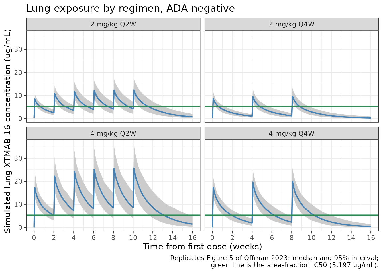
The paper concludes that 4 mg/kg Q2W keeps the median lung trough above the granuloma area-fraction IC50, while the other three regimens fall below it.
lung_trough_wk12 <- sim_fig5 |>
  dplyr::filter(time == week12) |>
  dplyr::group_by(regimen) |>
  dplyr::summarise(median_trough = median(Clung), .groups = "drop")
knitr::kable(
  lung_trough_wk12,
  digits = 2,
  caption = "Median simulated lung trough at week 12 (ug/mL)."
)| regimen | median_trough |
|---|---|
| 2 mg/kg Q2W | 4.13 |
| 2 mg/kg Q4W | 1.10 |
| 4 mg/kg Q2W | 8.67 |
| 4 mg/kg Q4W | 2.30 |
# The typical-value troughs are 7.7 (4 mg/kg Q2W) and 3.9, 2.1 and 1.1
# (the others), at least 25% from the IC50, so the cohort median cannot
# cross it through sampling noise.
med <- setNames(lung_trough_wk12$median_trough, lung_trough_wk12$regimen)
stopifnot(
  med[["4 mg/kg Q2W"]] > ic50_area_fraction,
  med[["2 mg/kg Q2W"]] < ic50_area_fraction,
  med[["2 mg/kg Q4W"]] < ic50_area_fraction,
  med[["4 mg/kg Q4W"]] < ic50_area_fraction
)
Assumptions and deviations
- No weight effect on clearance. The Discussion states that weight on CL, V and V2 was significant, but Supplementary Table S4 prints weight terms only on V and V2. The model follows Table S4: with CL independent of weight, the CL (0.129 mL/h/kg), AUCinf and Cavg values of Supplementary Tables S5 and S7 for a 70 kg subject are reproduced to the printed digits, which they would not be with an allometric term on CL.
-
Single weight exponent on both volumes. Table S4
prints the same exponent, 0.426, on V and V2; it is encoded as one
parameter (
e_wt_vc) applied to both. - Log-normal IIV. Table S4 reports the random effects as variances without stating the form; exponential (log-normal) IIV, the Phoenix NLME default for PK parameters, is assumed.
- Residual error. The proportional (6.89%) and additive (819 ng/mL) terms of Table S4 are taken as standard deviations and combined as variances (the nlmixr2 default combined error). The additive SD is converted to 0.819 mg/L to match the model’s mg/L concentration unit.
-
ADA covariate.
ADA_POSis the subject-level indicator of Table 1 (1 if any sample was ADA-positive). The study gave single doses only, and the paper’s dosing simulations, like the Figure 5 and Table S5/S6 checks here, use ADA-negative subjects. - Lung concentration is not part of the model. The paper derives lung interstitial concentrations by multiplying serum concentrations by the literature antibody biodistribution coefficient for lung (14.9%); this is a fixed post-processing factor rather than an estimated model component, so it is applied in this vignette rather than in the model file.
- Table S6 average-concentration column. In the lung table the repeated-dose “Cavg” values (2.40, 4.81, 0.91, 1.82 ug/mL) repeat the single-dose trough column and do not equal 14.9% of the serum Cavg in Table S5 (for example 0.149 x 46.1 = 6.87 ug/mL for 2 mg/kg Q2W). The column appears to be a transcription error in the supplement; only the lung troughs are compared here.
- In vitro concentration-response. The granuloma area-fraction and IL-1beta IC50s (5.197 and 3.465 ug/mL, Figure 3) come from curve fits whose other parameters and functional form are not reported; they are used here only as reference lines.
- Figure 5 interval width. The simulated medians match Figure 5, and so do the regimens whose trough crosses the IC50. The 97.5th percentile at the later 4 mg/kg Q2W peaks is wider than in the published figure, about 37 versus about 30 ug/mL read from the plot. The paper says only that the parameters were “obtained from sampling via the final PPK variance-covariance matrix”. It does not say whether the weight sampling, the omega matrix or the parameter uncertainty differ from the IIV-only, uniform 50-100 kg simulation used here, so the difference is not resolved.
- Figure 4 cohort. Body weight is drawn from a normal distribution with the Table 1 mean and SD, truncated to the observed range; ADA positivity is drawn at the observed 8 of 19.
- No correction notice for the article was found on Europe PMC as of 2026-10-26.