Paclitaxel and carboplatin myelosuppression in real-world use (Salem 2023)
Source:vignettes/articles/Salem_2023_paclitaxel.Rmd
Salem_2023_paclitaxel.RmdModel and source
- Citation: Salem AM, Dvergsten E, Karovic S, Maitland ML, Gopalakrishnan M. Model-based approach to identify predictors of paclitaxel-induced myelosuppression in ‘real-world’ administration. CPT Pharmacometrics Syst Pharmacol. 2023;12(7):929-940. doi:10.1002/psp4.12963. Model code and final estimates in Appendix S1 (Pumas code and fit output); equations, Table S1 and Figure S2 in Appendix S2. The fixed PK layers reproduce Joerger et al. Clin Cancer Res. 2006;12(7 Pt 1):2150-2157 (paclitaxel) and Joerger et al. Clin Cancer Res. 2007;13(21):6410-6418 (carboplatin), as transcribed in Appendix S1.
- Description: Semi-physiological (Friberg) PK/PD model of paclitaxel- and carboplatin-induced myelosuppression fitted to first-cycle absolute neutrophil counts from electronic health records of adults treated with weekly paclitaxel, weekly paclitaxel/carboplatin or every-3-weeks paclitaxel/carboplatin in routine care (Salem 2023, n = 405). The PK layers are fixed literature models: a three-compartment paclitaxel model with saturable elimination and saturable distribution to the first peripheral compartment (covariates body surface area, sex, total bilirubin and age), and a two-compartment linear carboplatin model. Both drug concentrations inhibit proliferation through multiplicative linear effects (1 - SLOPE * C); the PD parameters (baseline ANC, mean transit time, feedback exponent and both slopes) were estimated with log-normal IIV on baseline ANC, MTT and both slopes and a proportional residual error on ANC.
- Article: https://doi.org/10.1002/psp4.12963 (open access; the Pumas model code and fit output are Appendix S1, the equations, Table S1 and Figure S2 are Appendix S2)
Salem et al. applied published models to first-cycle absolute neutrophil counts (ANC) taken from electronic health records. Paclitaxel and carboplatin concentrations were never measured, so both PK layers are fixed literature models (paclitaxel from Joerger 2006, carboplatin from Joerger 2007), and only the Friberg myelosuppression parameters were estimated. The packaged model is this first approach (“PK fixed, PD estimated”), which the authors used for all downstream analyses.
Population
The analysis dataset held 405 adults treated at the Inova Schar Cancer Institute (Fairfax, Virginia) between 2015 and 2019 with weekly paclitaxel (n = 167), weekly paclitaxel/carboplatin (n = 179) or every-3-weeks paclitaxel/carboplatin (n = 59) (Table 1). 86.2% were women; 86 patients (21.2%) were 70 years or older and 20 (5%) were 80 or older. Breast cancer was the most common primary site (58.7%), followed by ovarian (8.1%) and non-small cell lung cancer (7.4%). 221 patients reported European ancestry, 55 Asian and 45 African American. The median paclitaxel dose was 80 mg/m^2 in the weekly regimens (1-h infusion) and 175 mg/m^2 every 3 weeks (3-h infusion); carboplatin was infused over 30 min. Mean baseline ANC was 7.4 and 6.9 x 10^9/L in patients younger and older than 70 years. 2274 ANC values were analysed (median 5 per patient).
The same information is available programmatically via
readModelDb("Salem_2023_paclitaxel")()$population.
Source trace
Every ini() value carries an in-file comment pointing at
its source. The estimates are taken from the Appendix S1 fit output,
which prints them to more digits than Table S1.
| Equation / parameter | Value | Source location |
|---|---|---|
lvc (paclitaxel Vc) |
12.8 L, fixed | Appendix S1 @pre; Figure S2A |
lvp2, e_bsa_vp2 (paclitaxel Vp) |
252 L x (BSA/1.8)^1.17, fixed | Appendix S1 @pre; Figure S2A |
lq2, e_bsa_q2 (paclitaxel Q) |
20.1 L/h x (BSA/1.8)^0.724, fixed | Appendix S1 @pre; Figure S2A |
lvmax, e_sexm_vmax,
e_bsa_vmax, e_tbili_vmax,
e_age_vmax (VMEL) |
37.4 umol/h x 1.2^SEX x (BSA/1.8)^0.842 x (BILI/7)^-0.167 x (AGE/56)^-0.352, fixed | Appendix S1 @pre; Figure S2A |
lkm (KMEL) |
0.53 umol/L, fixed | Appendix S1 @pre; Figure S2A |
lvmtr, e_sexm_vmtr,
e_bsa_vmtr (VMTR) |
169 umol/h x 1.2^SEX x (BSA/1.8)^0.911, fixed | Appendix S1 @pre; Figure S2A |
lkmtr, e_sexm_kmtr (KMTR) |
0.83 umol/L x 2.11^SEX, fixed | Appendix S1 @pre; Figure S2A |
lk21, e_sexm_k21 (K21) |
1.15 1/h x 0.893^SEX, fixed | Appendix S1 @pre; Figure S2A |
lcl_carboplatin, lvc_carboplatin,
lq_carboplatin, lvp_carboplatin
|
7.38 L/h, 11.9 L, 90.5 L/h, 8.23 L, fixed | Appendix S1 @pre; Figure S2A |
lcirc0 |
6.2787 x 10^9/L | Appendix S1 estimate; Table S1 (6.3, RSE 3%) |
lmtt |
143.71 h | Appendix S1 estimate; Table S1 (143.7, RSE 3%) |
gamma |
0.19585 | Appendix S1 estimate; Table S1 (0.2, RSE 6%) |
lslope |
5.8194 L/umol | Appendix S1 estimate; Table S1 (5.8, RSE 5.1%) |
lslope_carboplatin |
0.0058817 L/mg | Appendix S1 estimate; Table S1 (0.006, RSE 34.2%); unit see Assumptions |
etalcirc0, etalmtt,
etalslope
|
0.23317, 0.031576, 0.11131 | Appendix S1 Omega_1 (variances); Table S1 48.3, 17.7, 33.3 %CV |
etalslope_carboplatin |
3.3201 | Appendix S1 Omega_2; Table S1 182.2 %CV |
propSd |
0.36922 | Appendix S1 sigma_prop; Table S1 36.9% |
| Paclitaxel PK ODEs | n/a | Appendix S1 @dynamics; Appendix S2 Eqs. 1-3 |
| Carboplatin PK ODEs | n/a | Appendix S1 @dynamics
|
Friberg chain, ktr = 4 / MTT, edrug,
feedback |
n/a | Appendix S1 @vars / @dynamics; Appendix S2
Eqs. 4-11 |
| Initial conditions (all PD states = CIRC0) | n/a | Appendix S1 @init
|
ANC ~ prop(propSd) |
n/a | Appendix S1 @derived
|
Typical PK profiles (Figure S2B and S2C)
Figure S2 simulates the typical paclitaxel profile after a 3-h infusion of 175 mg/m^2 and the typical carboplatin profile after a 30-min infusion dosed to an AUC of 5 mg.min/mL. The typical patient below is a woman with BSA 1.8 m^2, total bilirubin 7 umol/L and age 56 years, the reference values of the paclitaxel covariate model. Paclitaxel doses enter in umol (molar mass 853.9 g/mol) and carboplatin doses in mg; with the model’s fixed carboplatin clearance of 7.38 L/h (123 mL/min) an AUC of 5 mg.min/mL needs 615 mg.
mod <- readModelDb("Salem_2023_paclitaxel")
mod_typ <- rxode2::zeroRe(mod)
#> ℹ parameter labels from comments will be replaced by 'label()'

mw_paclitaxel <- 853.9 # g/mol
umol_paclitaxel <- function(mg) mg / mw_paclitaxel * 1000
cl_carboplatin_ml_min <- 7.38 * 1000 / 60
calvert_mg <- function(auc) auc * cl_carboplatin_ml_min

dose_ptx <- umol_paclitaxel(175 * 1.8)
dose_carb <- calvert_mg(5)

ev_typ <- bind_rows(
  data.frame(time = 0, amt = dose_ptx, rate = dose_ptx / 3, cmt = "central", evid = 1),
  data.frame(time = 3, amt = dose_carb, rate = dose_carb / 0.5, cmt = "central_carboplatin", evid = 1),
  data.frame(time = sort(unique(c(seq(0, 12, by = 0.05), seq(12, 80, by = 0.5)))),
             amt = 0, rate = 0, cmt = "central", evid = 0)
) |>
  mutate(id = 1L, BSA = 1.8, SEXF = 1, TBILI = 7, AGE = 56) |>
  arrange(time, desc(evid))

sim_typ <- as.data.frame(rxode2::rxSolve(mod_typ, ev_typ, returnType = "data.frame"))
#> ℹ omega/sigma items treated as zero: 'etalcirc0', 'etalmtt', 'etalslope', 'etalslope_carboplatin'
sim_typ |>
  transmute(
    time,
    `Paclitaxel (umol/L)` = Cc,
    `Carboplatin (mg/L), dosed at t = 3 h` = Cc_carboplatin
  ) |>
  pivot_longer(-time, names_to = "analyte", values_to = "conc") |>
  filter(conc > 1e-3) |>
  ggplot(aes(time, conc)) +
  geom_line(colour = "navy") +
  facet_wrap(~analyte, scales = "free") +
  scale_y_log10() +
  labs(x = "Time (h)", y = "Concentration",
       caption = "Replicates Figure S2B (paclitaxel) and S2C (carboplatin) of Salem 2023.")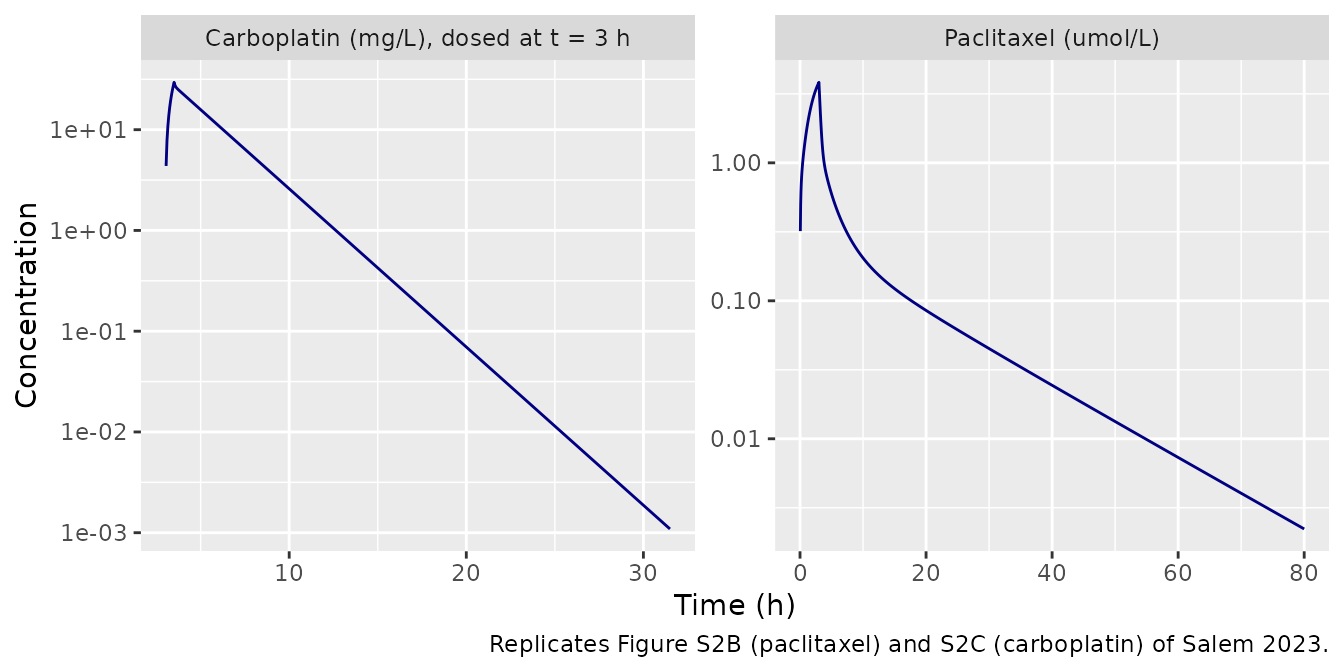
The figure’s carboplatin panel starts at the carboplatin dose; here the carboplatin infusion follows the 3-h paclitaxel infusion, so its curve is shifted by 3 h.
PKNCA comparison with Figure S2
The reference values were read by the maintainers from Figure S2: the paclitaxel peak sits about 0.6 decades above the 1 umol/L gridline (about 4 umol/L), and the carboplatin peak at about 27.5 mg/L. The carboplatin AUC reference is the dosing target itself (5 mg.min/mL = 83.3 mg.h/L).
nca_typ_conc <- bind_rows(
  sim_typ |> transmute(id = 1L, time, Cc, analyte = "paclitaxel"),
  sim_typ |> transmute(id = 1L, time = time - 3, Cc = Cc_carboplatin, analyte = "carboplatin") |>
    filter(time >= 0)
) |>
  filter(!is.na(Cc))
stopifnot(all(c(0) %in% nca_typ_conc$time))
nca_typ_dose <- data.frame(
  id = 1L, time = 0, amt = c(dose_ptx, dose_carb),
  analyte = c("paclitaxel", "carboplatin")
)
nca_typ <- PKNCA::pk.nca(PKNCA::PKNCAdata(
  PKNCA::PKNCAconc(nca_typ_conc, Cc ~ time | analyte + id),
  PKNCA::PKNCAdose(nca_typ_dose, amt ~ time | analyte + id),
  intervals = data.frame(start = 0, end = Inf, cmax = TRUE, aucinf.obs = TRUE)
))

published_typ <- tibble::tribble(
  ~analyte, ~cmax, ~aucinf.obs,
  "paclitaxel", 4.0, NA,
  "carboplatin", 27.5, 5 * 1000 / 60
)
cmp_typ <- nlmixr2lib::ncaComparisonTable(
  simulated = nca_typ,
  reference = published_typ,
  by = "analyte",
  units = c(cmax = "umol/L paclitaxel, mg/L carboplatin",
            aucinf.obs = "umol*h/L paclitaxel, mg*h/L carboplatin"),
  tolerance_pct = 20
)
knitr::kable(cmp_typ, caption = "Typical-patient PK: simulated (PKNCA) vs. Figure S2. * differs by > 20%.")| NCA parameter | analyte | Reference | Simulated | % diff |
|---|---|---|---|---|
| Cmax (umol/L paclitaxel, mg/L carboplatin) | paclitaxel | 4 | 3.83 | -4.2% |
| Cmax (umol/L paclitaxel, mg/L carboplatin) | carboplatin | 27.5 | 29.5 | +7.3% |
| AUC0-∞ (obs) (umolh/L paclitaxel, mgh/L carboplatin) | paclitaxel | — | 13.5 | — |
| AUC0-∞ (obs) (umolh/L paclitaxel, mgh/L carboplatin) | carboplatin | 83.3 | 83.3 | -0.0% |
res_typ <- as.data.frame(nca_typ$result)
pk_val <- function(an, p) {
  v <- res_typ$PPORRES[res_typ$analyte == an & res_typ$PPTESTCD == p]
  if (length(v) != 1L) stop("no unique PKNCA row for ", an, " ", p)
  v
}
# Paclitaxel tail read from Figure S2B: about 0.09 umol/L at 20 h and
# 0.0025 umol/L at 80 h. These are deterministic typical-value solves, so the
# tolerance only has to cover the reading of a log-scale figure.
c20 <- sim_typ$Cc[sim_typ$time == 20]
c80 <- sim_typ$Cc[sim_typ$time == 80]
stopifnot(
  abs(pk_val("paclitaxel", "cmax") / 4.0 - 1) < 0.15,
  abs(c20 / 0.09 - 1) < 0.25,
  abs(c80 / 0.0025 - 1) < 0.30,
  abs(pk_val("carboplatin", "cmax") / 27.5 - 1) < 0.15,
  # Linear carboplatin: AUC = dose / CL exactly; only integration error remains.
  abs(pk_val("carboplatin", "aucinf.obs") / (dose_carb / 7.38) - 1) < 0.01
)
Both typical profiles agree with Figure S2: the paclitaxel peak is 3.83 umol/L and the concentration at 20 h is 0.085 umol/L; the carboplatin peak is 29.5 mg/L. The carboplatin match is also the evidence for its concentration unit (see Assumptions).
Virtual cohort
Patient-level data are not public. The cohort below approximates Table 1: 86% women, BSA about 1.8 m^2 (SD 0.22), total bilirubin log-normal with mean 8.6 umol/L (SD 4.5), and age normal with mean 60 years (SD 12) truncated to 18-90 years, which puts about 20% of patients at 70 years or older (the paper reports 21.2% but not the mean age). Each regimen gets 150 patients.
set.seed(2023)
rxode2::rxSetSeed(2023)

n_per_arm <- 150L
regimens <- tibble::tribble(
  ~regimen, ~ptx_mg_m2, ~ptx_inf_h, ~carb_auc, ~dose_days,
  "Weekly paclitaxel", 80, 1, 0, list(c(0, 7, 14, 21)),
  "Weekly paclitaxel/carboplatin", 80, 1, 2, list(c(0, 7, 14, 21)),
  "Every 3 weeks paclitaxel/carboplatin", 175, 3, 5, list(0)
)

rtrunc_norm <- function(n, mean, sd, lo, hi) {
  x <- rnorm(n, mean, sd)
  bad <- x < lo | x > hi
  while (any(bad)) {
    x[bad] <- rnorm(sum(bad), mean, sd)
    bad <- x < lo | x > hi
  }
  x
}

# Dose and observation rows for one regimen, given one row per subject.
regimen_events <- function(reg, subj) {
  days <- unlist(reg$dose_days)
  doses <- subj |>
    tidyr::expand_grid(day = days) |>
    mutate(time = day * 24, amt = umol_paclitaxel(reg$ptx_mg_m2 * BSA),
           rate = amt / reg$ptx_inf_h, cmt = "central", evid = 1)
  if (reg$carb_auc > 0) {
    carb <- subj |>
      tidyr::expand_grid(day = days) |>
      mutate(time = day * 24 + reg$ptx_inf_h, amt = calvert_mg(reg$carb_auc),
             rate = amt / 0.5, cmt = "central_carboplatin", evid = 1)
    doses <- bind_rows(doses, carb)
  }
  obs_times <- sort(unique(c(seq(0, 12, by = 0.25), seq(12, 28 * 24, by = 6))))
  obs <- subj |>
    tidyr::expand_grid(time = obs_times) |>
    mutate(amt = 0, rate = 0, cmt = "central", evid = 0)
  bind_rows(doses, obs) |>
    select(-any_of("day")) |>
    arrange(id, time, desc(evid))
}

make_cohort <- function(reg, id_offset) {
  n <- n_per_arm
  subj <- tibble(
    id = id_offset + seq_len(n),
    regimen = reg$regimen,
    SEXF = rbinom(n, 1, 0.862),
    BSA = rtrunc_norm(n, 1.8, 0.22, 1.3, 2.6),
    TBILI = rlnorm(n, log(8.6) - 0.5 * log(1 + (4.5 / 8.6)^2), sqrt(log(1 + (4.5 / 8.6)^2))),
    AGE = rtrunc_norm(n, 60, 12, 18, 90)
  )
  regimen_events(reg, subj)
}

events <- bind_rows(lapply(seq_len(nrow(regimens)), function(i) {
  make_cohort(regimens[i, ], id_offset = (i - 1L) * n_per_arm)
}))
stopifnot(!anyDuplicated(unique(events[, c("id", "time", "evid", "cmt")])))
Simulation
sim <- rxode2::rxSolve(mod, events = events, keep = c("regimen", "AGE")) |>
  as.data.frame() |>
  mutate(regimen = factor(regimen, levels = regimens$regimen))
#> ℹ parameter labels from comments will be replaced by 'label()'
stopifnot(!anyNA(sim$ANC))
ANC over the first month (Figure S4)
sim |>
  group_by(regimen, time) |>
  summarise(
    Q05 = quantile(ANC, 0.05), Q50 = quantile(ANC, 0.5), Q95 = quantile(ANC, 0.95),
    .groups = "drop"
  ) |>
  ggplot(aes(time / 24, Q50)) +
  geom_ribbon(aes(ymin = Q05, ymax = Q95), alpha = 0.25, fill = "firebrick") +
  geom_line(colour = "firebrick") +
  facet_wrap(~regimen, ncol = 1) +
  labs(x = "Time after first dose (days)", y = "ANC (10^9 cells/L)",
       caption = "Median and 5th-95th percentiles of simulated ANC; compare Figure S4 of Salem 2023.")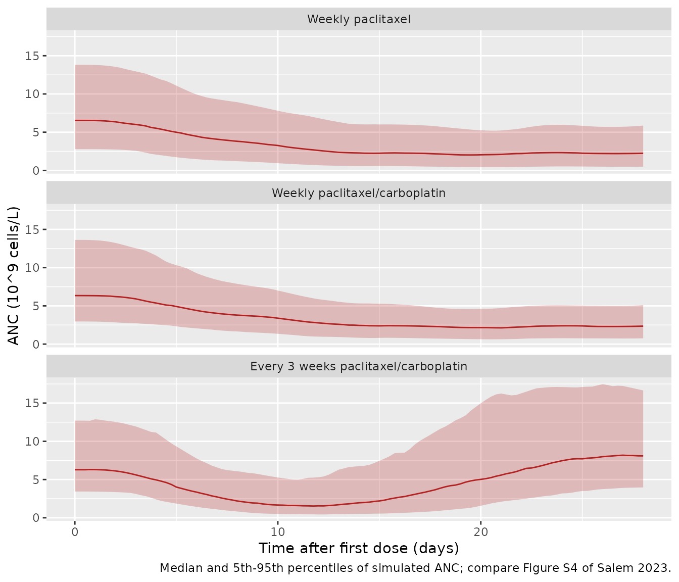
Nadir ANC by regimen and age (Figure 3)
The paper reports the mean model-predicted (individual) nadir ANC during the first month: 2.09, 2.81 and 2.45 x 10^9/L for every-3-weeks paclitaxel/carboplatin, weekly paclitaxel/carboplatin and weekly paclitaxel, and 2.6 and 2.4 x 10^9/L for patients younger and older than 70 years.
nadir <- sim |>
  group_by(id, regimen, AGE) |>
  summarise(nadir = min(ANC), .groups = "drop") |>
  mutate(age_group = ifelse(AGE >= 70, ">= 70 years", "< 70 years"))

published_nadir <- tibble::tribble(
  ~regimen, ~published,
  "Every 3 weeks paclitaxel/carboplatin", 2.09,
  "Weekly paclitaxel/carboplatin", 2.81,
  "Weekly paclitaxel", 2.45
)
nadir_tab <- nadir |>
  group_by(regimen) |>
  summarise(simulated_mean = mean(nadir), simulated_median = median(nadir), .groups = "drop") |>
  mutate(regimen = as.character(regimen)) |>
  inner_join(published_nadir, by = "regimen") |>
  mutate(pct_diff = 100 * (simulated_mean / published - 1))
stopifnot(nrow(nadir_tab) == 3L)

nadir_tab |>
  rename(
    Regimen = regimen,
    "Simulated mean nadir (10^9/L)" = simulated_mean,
    "Simulated median nadir (10^9/L)" = simulated_median,
    "Published mean predicted nadir (10^9/L)" = published,
    "Difference (%)" = pct_diff
  ) |>
knitr::kable(digits = 2, caption = "First-month nadir ANC by regimen.")| Regimen | Simulated mean nadir (10^9/L) | Simulated median nadir (10^9/L) | Published mean predicted nadir (10^9/L) | Difference (%) |
|---|---|---|---|---|
| Weekly paclitaxel | 2.31 | 1.92 | 2.45 | -5.83 |
| Weekly paclitaxel/carboplatin | 2.28 | 2.06 | 2.81 | -18.82 |
| Every 3 weeks paclitaxel/carboplatin | 1.78 | 1.43 | 2.09 | -14.99 |
The simulated cohort means differ from the published means by -19% to -6%. The every-3-weeks regimen gives the deepest nadir in both. Weekly paclitaxel with and without carboplatin come out almost equal in the simulation, while the published means put the carboplatin arm higher. The real arms differ in ways a common virtual cohort does not carry: 24% of the weekly paclitaxel/carboplatin patients were 70 or older against 14% of the weekly paclitaxel patients (Table 1), and weekly paclitaxel was the usual breast cancer regimen while weekly paclitaxel/carboplatin was the usual lung cancer regimen (Results).
ggplot(nadir, aes(age_group, nadir)) +
  geom_boxplot(outlier.size = 0.5) +
  facet_wrap(~regimen) +
  labs(x = NULL, y = "Nadir ANC (10^9 cells/L)",
       caption = "Simulated first-month nadir ANC by age group; compare Figure 3 of Salem 2023.")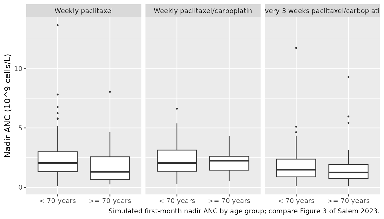
# The cohort mean nadir differs from the published means for reasons that
# move every arm by a similar amount (the virtual cohort's baseline ANC is
# the model's log-normal CIRC0, while the published means are individual
# predictions in the observed cohort), so the gate is on the centre of the
# three differences, not on each arm. A mis-transcribed slope, MTT or dose
# unit moves the nadir by far more than this.
stopifnot(
  abs(median(nadir_tab$pct_diff)) < 30,
  all(nadir_tab$simulated_mean > 0.5), all(nadir_tab$simulated_mean < 6)
)
The age effect enters the model only through the paclitaxel VMEL exponent (-0.352): older patients clear paclitaxel more slowly and so reach a somewhat lower nadir. The paper’s mean predicted nadirs (2.6 vs. 2.4 x 10^9/L below and above 70 years) and its regression analysis found no meaningful age effect. For the typical every-3-weeks patient:
# Typical-value first-month nadir for one regimen: a woman with BSA 1.8 m^2
# and total bilirubin 7 umol/L.
typ_nadir <- function(regimen, age = 56, mod_use = mod_typ) {
  reg <- regimens[regimens$regimen == regimen, ]
  stopifnot(nrow(reg) == 1L)
  subj <- tibble(id = 1L, regimen = regimen, SEXF = 1, BSA = 1.8, TBILI = 7, AGE = age)
  ev <- regimen_events(reg, subj)
  min(as.data.frame(rxode2::rxSolve(mod_use, ev, returnType = "data.frame"))$ANC)
}
q3w <- "Every 3 weeks paclitaxel/carboplatin"
age_eff <- c(age50 = typ_nadir(q3w, 50), age80 = typ_nadir(q3w, 80))
age_eff
#>    age50    age80
#> 1.328128 1.061601
# Deterministic typical-value solves: the VMEL age exponent moves the nadir
# by well under 1 x 10^9/L across 50-80 years.
stopifnot(abs(age_eff[["age80"]] - age_eff[["age50"]]) < 1)
Literature PD parameters (external-validation approach)
In their second approach the authors fixed the PD parameters as well, to the literature values that also served as initial estimates in Appendix S1 (CIRC0 4.35 x 10^9/L, MTT 141 h, gamma 0.26, SLOPE 2.08, SLOPEC 0.00162). They report that both approaches fit the ANC data similarly (Figure S6), with the estimated slopes about 2.8-fold (paclitaxel) and 3-fold (carboplatin) higher than the literature values because typical rather than individual PK was used. The typical nadirs under both parameter sets:
mod_lit <- mod_typ |>
  rxode2::ini(
    lcirc0 = log(4.35), lmtt = log(141), gamma = 0.26,
    lslope = log(2.08), lslope_carboplatin = log(0.00162)
  )
lit_tab <- tibble(
  regimen = regimens$regimen,
  estimated = vapply(regimen, typ_nadir, numeric(1)),
  literature = vapply(regimen, typ_nadir, numeric(1), mod_use = mod_lit)
)
lit_tab |>
  rename(
    Regimen = regimen,
    "Typical nadir, estimated PD (10^9/L)" = estimated,
    "Typical nadir, literature PD (10^9/L)" = literature
  ) |>
knitr::kable(digits = 2, caption = "Typical-patient first-month nadir ANC under the estimated and the literature PD parameters.")| Regimen | Typical nadir, estimated PD (10^9/L) | Typical nadir, literature PD (10^9/L) |
|---|---|---|
| Weekly paclitaxel | 1.96 | 3.13 |
| Weekly paclitaxel/carboplatin | 1.98 | 3.13 |
| Every 3 weeks paclitaxel/carboplatin | 1.26 | 2.40 |
PKNCA of the first paclitaxel and carboplatin doses
The paper reports no NCA. For completeness, the first-week exposure of each regimen in the virtual cohort:
conc_ptx <- sim |>
  filter(!is.na(Cc), time <= 168) |>
  select(id, time, Cc, regimen) |>
  mutate(regimen = as.character(regimen))
stopifnot(all(tapply(conc_ptx$time, conc_ptx$id, min) == 0))
dose_ptx_df <- events |>
  filter(evid == 1, cmt == "central", time == 0) |>
  select(id, time, amt, regimen)
nca_ptx <- PKNCA::pk.nca(PKNCA::PKNCAdata(
  PKNCA::PKNCAconc(conc_ptx, Cc ~ time | regimen + id),
  PKNCA::PKNCAdose(dose_ptx_df, amt ~ time | regimen + id),
  intervals = data.frame(start = 0, end = 168, cmax = TRUE, tmax = TRUE, auclast = TRUE)
))

# Carboplatin starts at the end of the paclitaxel infusion; time is taken
# from the carboplatin dose. Its 0.07 h half-life takes the tail into
# integrator noise within a day, where tiny negative values would make the
# log-down trapezoid return NaN, so the tail below 1e-6 of each subject's
# peak is dropped after checking it is noise.
conc_carb <- sim |>
  filter(!is.na(Cc_carboplatin), regimen != "Weekly paclitaxel") |>
  mutate(t_carb = time - ifelse(regimen == q3w, 3, 1)) |>
  filter(t_carb >= 0, t_carb <= 167) |>
  transmute(id, time = t_carb, Cc = Cc_carboplatin, regimen = as.character(regimen))
stopifnot(all(conc_carb$Cc >= -1e-6 * max(conc_carb$Cc)))
conc_carb <- conc_carb |>
  mutate(Cc = pmax(Cc, 0)) |>
  group_by(id) |>
  filter(time <= time[which.max(Cc)] | Cc >= 1e-6 * max(Cc)) |>
  ungroup()
dose_carb_df <- events |>
  filter(evid == 1, cmt == "central_carboplatin", time < 168) |>
  mutate(time = 0) |>
  select(id, time, amt, regimen)
nca_carb <- PKNCA::pk.nca(PKNCA::PKNCAdata(
  PKNCA::PKNCAconc(conc_carb, Cc ~ time | regimen + id),
  PKNCA::PKNCAdose(dose_carb_df, amt ~ time | regimen + id),
  intervals = data.frame(start = 0, end = Inf, cmax = TRUE, auclast = TRUE)
))
# Linear carboplatin: AUC = dose / CL for every subject; only integration
# error separates them.
res_carb <- as.data.frame(nca_carb$result) |>
  filter(PPTESTCD == "auclast") |>
  inner_join(dose_carb_df |> select(id, amt), by = "id")
stopifnot(nrow(res_carb) == 2L * n_per_arm,
          max(abs(res_carb$PPORRES / (res_carb$amt / 7.38) - 1)) < 0.01)

summarise_nca <- function(res, analyte) {
  as.data.frame(res$result) |>
    group_by(regimen, PPTESTCD) |>
    summarise(median = median(PPORRES), .groups = "drop") |>
    pivot_wider(names_from = PPTESTCD, values_from = median) |>
    mutate(analyte = analyte, .before = 1)
}
bind_rows(summarise_nca(nca_ptx, "paclitaxel (umol/L, umol*h/L)"),
          summarise_nca(nca_carb, "carboplatin (mg/L, mg*h/L)")) |>
  rename(
    Analyte = analyte, Regimen = regimen,
    "Median Cmax" = cmax, "Median AUClast (first dose)" = auclast, "Median Tmax (h)" = tmax
  ) |>
knitr::kable(digits = 3, caption = "Median first-week NCA in the virtual cohort.")| Analyte | Regimen | Median AUClast (first dose) | Median Cmax | Median Tmax (h) |
|---|---|---|---|---|
| paclitaxel (umol/L, umol*h/L) | Every 3 weeks paclitaxel/carboplatin | 13.818 | 3.857 | 3 |
| paclitaxel (umol/L, umol*h/L) | Weekly paclitaxel | 4.762 | 2.947 | 1 |
| paclitaxel (umol/L, umol*h/L) | Weekly paclitaxel/carboplatin | 4.730 | 2.891 | 1 |
| carboplatin (mg/L, mg*h/L) | Every 3 weeks paclitaxel/carboplatin | 83.269 | 29.510 | NA |
| carboplatin (mg/L, mg*h/L) | Weekly paclitaxel/carboplatin | 33.308 | 11.804 | NA |
Assumptions and deviations
- Carboplatin concentration unit. Table S1 labels the carboplatin slope SLOPEC in L/umol, but Figure S2C plots the authors’ simulated carboplatin profile in mg/L, and that profile is reproduced here only when carboplatin doses and concentrations are in mg and mg/L (a 615 mg dose for AUC 5 gives a peak of about 29 mg/L, against about 27.5 mg/L in the figure; in umol the peak would be about 2.7-fold higher). The maintainers therefore treat the carboplatin dose as mg and SLOPEC as L/mg, and read the Table S1 unit as carried over from the paclitaxel row. If the fit actually used molar carboplatin concentrations, multiply SLOPEC by 371.25 / 1000 (that is, give doses in umol) to recover it. Paclitaxel is in umol and umol/L in both Table S1 and Figure S2B, and its fixed PK parameters are stated in umol. The source of the carboplatin PK, Joerger 2007 (doi:10.1158/1078-0432.CCR-07-0064), states the unit the carboplatin model was built in and would settle the question; the maintainers kept mg/L (2026-11-06) and will re-check the unit against that paper.
- Sign of the saturable transfer in the central-compartment equation. Appendix S2 Eq. 1 prints the central -> first-peripheral Michaelis-Menten term with a plus sign; the Appendix S1 code, which is what was fitted, subtracts it, and only that form conserves mass. The model follows the code.
- No paclitaxel or carboplatin IIV. As in the source, both PK layers are typical-value models with covariates; the authors deliberately used typical rather than individual PK because no concentrations were measured.
-
The drug effect is not bounded.
edrug = 1 - SLOPE * Cbecomes negative at paclitaxel concentrations above 1 / 5.82 = 0.17 umol/L, which every regimen exceeds near the end of the infusion. This is the source’s linear model; proliferation then simply turns into net loss. - Regression analysis not encoded. Table 2 relates the post hoc random effects and nadirs to baseline ANC and regimen with a stepwise linear regression. Those are summaries of individual estimates, not covariates of the fitted model, and are not part of the packaged model.
- Virtual cohort and dosing. The paper gives Table 1 summaries by age group only, so the age distribution (normal, mean 60, SD 12, truncated 18-90 years) and the bilirubin distribution are maintainers’ choices. Carboplatin doses are not reported; the cohort uses AUC 2 weekly and AUC 5 every three weeks, dosed against the model’s fixed carboplatin clearance. Weekly regimens are dosed on days 0, 7, 14 and 21 and the every-3-weeks regimen on day 0, and the nadir is the minimum over 28 days. Carboplatin starts at the end of the paclitaxel infusion.
- Nadir comparison. The published nadirs are means of individual predictions in the real cohort, whose mean baseline ANC (about 7.3 x 10^9/L) differs from the cohort simulated from the model’s CIRC0 distribution; the comparison is a plausibility check on the centre, not a reproduction of individual fits.
- Errata. No correction notice for this article was found as of 2026-10-26.