S-ketamine + norketamine + ticlopidine DDI (Ashraf 2018)
Source:vignettes/articles/Ashraf_2018_s_ketamine_ticlopidine.Rmd
Ashraf_2018_s_ketamine_ticlopidine.RmdModel and source
MODEL <- "Ashraf_2018_s_ketamine_ticlopidine"
ui <- rxode2::rxode(readModelDb(MODEL))
#> ℹ parameter labels from comments will be replaced by 'label()'- Citation: Ashraf MW, Peltoniemi MA, Olkkola KT, Neuvonen PJ, Saari TI. Semimechanistic Population Pharmacokinetic Model to Predict the Drug-Drug Interaction Between S-ketamine and Ticlopidine in Healthy Human Volunteers. CPT Pharmacometrics Syst Pharmacol. 2018;7(10):687-697. doi:10.1002/psp4.12346
- Article: https://doi.org/10.1002/psp4.12346
- Supplementary Information S1 (study descriptions), S2 (model development and equations) and S3 (the final NONMEM control stream) are open access on the journal site and were the primary source for the ODE system and for every fixed constant.
Semi-PBPK. Joint semi-mechanistic population PK model of oral and intravenous S-ketamine, its primary metabolite norketamine, and the co-administered CYP2B6 mechanism-based inhibitor ticlopidine, with a mechanistic-static drug-drug-interaction layer, in healthy adult volunteers (Ashraf 2018). S-ketamine has three-compartment mammillary disposition with first-order absorption; norketamine has two-compartment disposition; ticlopidine has two-compartment disposition behind a four-transit absorption chain. All three compounds are eliminated by well-stirred gut-wall and hepatic clearance driven by weight-scaled physiological blood flows (QH = 3.75 * WT^0.75 L/h), with the S-ketamine gut wall additionally using the QGUT permeability model. For S-ketamine and norketamine the gut wall, portal vein and liver are solved by the simplified quasi-steady-state approximation (algebraic, not ODE states); for ticlopidine they are explicit ODE states because the portal-vein inhibitor concentration drives the interaction. All S-ketamine extracted at the gut wall and liver becomes norketamine (Fmet fixed to 1), so the norketamine disposition parameters are apparent. Ticlopidine inhibits hepatic CYP2B6 through the mechanistic static model: a reversible component AH = 1 / (1 + IPV / ki) and a time-dependent component BH = kdeg / (kdeg + kinact * IPV / (KI + IPV)) combine as fCLint = AH * BH * fm2B6 + (1 - fm2B6), which multiplies the S-ketamine intrinsic hepatic clearance. With no ticlopidine present the interaction term is exactly 1. Enzyme inactivation constants are in-vitro values fixed from Obach 2007; the CYP2B6-metabolised fraction 0.63 was estimated by log-likelihood profiling. No inhibition model is applied to norketamine or to ticlopidine’s own (auto-inhibited) metabolism because neither could be supported by the data.
Population
Concentration-time data were pooled from the placebo phases of five randomised, placebo-controlled, crossover healthy-volunteer studies run in Turku, Finland between June 2008 and March 2010, plus the complete placebo-and-ticlopidine dataset of the ticlopidine interaction study (Peltoniemi 2011). Forty-one non-smoking volunteers (21 male, 20 female) aged 19-35 years and weighing 50-88 kg took part; 13 of them participated in two studies and one in three, and repeat participations were modelled as separate individuals because the data could not support inter-occasion variability (Supplementary Information S1 footnote).
S-ketamine was given as a 0.2-0.3 mg/kg oral syrup, and as a 0.1 mg/kg intravenous injection over 2 minutes in the intravenous part of Study IV. Ticlopidine was given as 250 mg twice daily (08:00 and 20:00) for six days before the study day, with the last pre-treatment dose at 08:00 and S-ketamine one hour later at 09:00. Thirteen plasma samples per profile were drawn from pre-dose to 24 h; the goodness-of-fit figure reports 67 placebo-phase and 11 ticlopidine-phase S-ketamine / norketamine profiles.
str(ui$population, max.level = 1)
#> List of 12
#>  $ species       : chr "human"
#>  $ n_subjects    : int 41
#>  $ n_studies     : int 5
#>  $ age_range     : chr "19-35 years (per-study means 22.0-27.5 years)"
#>  $ weight_range  : chr "50-88 kg (per-study means 59-70 kg)"
#>  $ sex_female_pct: num 48.8
#>  $ disease_state : chr "Healthy, non-smoking adult volunteers; no concomitant drug therapy for at least 14 days before study entry and "| __truncated__
#>  $ dose_range    : chr "S-ketamine 0.2-0.3 mg/kg as an oral syrup (Studies I, II, III, IV oral part, V) and 0.1 mg/kg intravenously ove"| __truncated__
#>  $ regions       : chr "Single centre, Turku, Finland (clinical phases run June 2008 - March 2010)."
#>  $ co_medication : chr "None permitted. The ticlopidine phase of Study III is the only interaction arm carried into this model; the cla"| __truncated__
#>  $ n_observations: chr "13 timed plasma samples per individual (pre-dose and 20 min, 40 min, 1, 1.5, 2, 3, 4, 5, 6, 8, 10, 12 and 24 h "| __truncated__
#>  $ notes         : chr "Data pooled from the placebo phases of five randomised, placebo-controlled, crossover healthy-volunteer studies"| __truncated__
Source trace
Every value is traced in-file next to its ini() entry in
inst/modeldb/specificDrugs/Ashraf_2018_s_ketamine_ticlopidine.R.
The table collects them here. “S3” is the deposited final NONMEM control
stream and “S2” is the model-development supplement.
| Quantity | Value | Source |
|---|---|---|
lka, lvc, lq,
lvp, lq2, lvp2
|
1.76 /h; 14.4, 287, 102, 22.4, 180 L or L/h | Table 2, S-ketamine block |
lclint_liver, lclint_gut
|
301, 1.19 L/h | Table 2, CL INT,H,SK / CL INT,GW,SK
|
clperm |
4.1 L/h (fixed) | S3 $THETA 9 = 4.1 FIX; derived in S2 from a PAMPA
Papp of 1.49e-6 cm/s |
dur_iv |
0.03333 h (fixed) | S3 $PK D2 = 0.03333 (2-minute i.v. injection) |
lvc_snk, lq_snk, lvp_snk
|
88.4, 19.9, 88.9 | Table 2, norketamine block (apparent; footnote b) |
lclint_liver_snk, lclint_gut_snk
|
73.5, 44.4 L/h | Table 2, CL INT,H,NK / CL INT,GW,NK
|
lka_tic |
3.3 /h (fixed) | Table 2 K a,TIC (FIXED); S3
$THETA 15 = 3.3 FIX
|
lvc_tic, lq_tic, lvp_tic,
lclint_liver_tic
|
50.3, 26.3, 191, 1505 | Table 2, ticlopidine block |
clint_gut_tic |
0 (fixed) | Table 2 CL INT,GW,TIC = 0 (FIXED); S3
$THETA 20 = 0 FIX
|
fu, fu_snk, fu_tic
|
0.70, 0.50, 0.02 | Table 1 |
bp, bp_snk, bp_tic
|
0.50, 1, 1 | Table 1 BP RATIO
|
fu_gut, fu_gut_snk,
fu_gut_tic
|
1, 1, 1 | Table 1 |
qh_coef, e_wt_qh
|
3.75, 0.75 | Table 1 Q H = 3.75 * WTKG^0.75
|
fq_portal, fq_hepatic_artery,
fq_intestinal, fq_mucosal,
fq_villous
|
0.75, 0.25, 0.40, 0.80, 0.60 | Table 1 |
vgut, vportal, vliver
|
1, 1, 1 L | Table 1 |
kirev_2b6 (ki) |
0.031 umol/L (fixed) | Table 1; S3 $THETA 25 (control-stream
TKIN) |
ki_2b6 (KI) |
0.57 umol/L (fixed) | Table 1; S3 $THETA 21
|
kinact_2b6 |
18 /h (fixed) | Table 1 k inact = 0.30 /min; S3
$THETA 22 = 18 FIX
|
kdeg_2b6 |
0.017 /h (fixed) | S3 $THETA 24 = 0.017 FIX; see Errata |
fm_cyp2b6 |
0.63 (fixed) | Table 1 footnote, Results; S3 $THETA 23 = 0.63 FIX
|
| IIV variances | 0.25, 2.1, 0.42, 0.045, 0.10, 0.12 | Table 2 IIV on ... rows |
| Residual variances | 0.086, 0.065, 0.062, 0.064, 0.066 | Table 2 RV ... rows (NONMEM $SIGMA
variances) |
| Well-stirred gut / hepatic availability | equations | S2 F_H = Q_H / (Q_H + fu * CL_INT,H) and the gut-wall
analogue |
QGUT model |
qgut = qvi * clperm / (qvi + clperm) |
S3 $PK QGUT; S2 “QGUT-model” |
| Quasi-steady-state gut / portal / liver amounts | equations | S2 S-ketamine and norketamine equation blocks; S3
$DES
|
| Ticlopidine transit + gut / portal / liver ODEs | equations | S2 ticlopidine equation block; S3 $DES
|
AH, BH, fCL'int,H,
CLint,H,[I]
|
equations | S2 “Drug-drug interaction model”; S3 $DES
TAH / TBH / ZETA
|
%RA = AH * BH * Activity[I]=0 |
equation | Results, “Simulations” |
Structural verification
The model has an exact closed form for every steady-state clearance
and availability, so the ODE transcription can be checked against
arithmetic rather than against a picture. All of the checks below use
the typical subject (rxode2::zeroRe()), so
they are deterministic and are asserted tightly.
WT_REF <- 70

p <- as.list(setNames(ui$theta, names(ui$theta)))
qh <- exp(0) * 3.75 * WT_REF^0.75 # Table 1
qvi <- 0.60 * 0.80 * 0.40 * qh # villous <- mucosal <- intestinal <- hepatic
fub <- 0.70 / 0.50 # S-ketamine unbound fraction in blood
fub_snk <- 0.50 / 1
fub_tic <- 0.02 / 1

qgut <- qvi * 4.1 / (qvi + 4.1)
fgut <- qgut / (qgut + 1.19 * 1)
fliver <- qh / (qh + fub * 301)
cl_sk <- (1 - fliver) * qh # well-stirred hepatic clearance
f_po <- fgut * fliver # oral bioavailability

fgut_snk <- qvi / (qvi + 44.4 * 1)
fliver_snk <- qh / (qh + fub_snk * 73.5)
cl_snk <- (1 - fliver_snk) * qh

fliver_tic <- qh / (qh + fub_tic * 1505)
cl_tic <- (1 - fliver_tic) * qh

tibble::tibble(
  Quantity = c(
    "QH (L/h)", "QVI (L/h)", "QGUT (L/h)",
    "FGW,SK", "FH,SK", "CL_SK (L/h)", "F oral (SK)",
    "FGW,NK", "FH,NK", "CL_NK (L/h)",
    "FH,TIC", "CL_TIC (L/h)"
  ),
  Value = c(qh, qvi, qgut, fgut, fliver, cl_sk, f_po, fgut_snk, fliver_snk, cl_snk, fliver_tic, cl_tic)
) |>
knitr::kable(digits = 4, caption = "Closed-form quantities at 70 kg, no inhibitor.")| Quantity | Value |
|---|---|
| QH (L/h) | 90.7517 |
| QVI (L/h) | 17.4243 |
| QGUT (L/h) | 3.3190 |
| FGW,SK | 0.7361 |
| FH,SK | 0.1772 |
| CL_SK (L/h) | 74.6708 |
| F oral (SK) | 0.1304 |
| FGW,NK | 0.2818 |
| FH,NK | 0.7118 |
| CL_NK (L/h) | 26.1575 |
| FH,TIC | 0.7509 |
| CL_TIC (L/h) | 22.6031 |
ui_typ <- rxode2::zeroRe(ui)

# Dense early grid (absorption + fast distribution) then a long tail so the
# trapezoidal AUC is effectively AUC(0-inf).
GRID <- sort(unique(c(seq(0, 4, 0.001), seq(4, 48, 0.005), seq(48, 1500, 0.05))))

trap <- function(t, y) sum(diff(t) * (head(y, -1) + tail(y, -1)) / 2)

solve_typical <- function(cmt, amt, rate = 0, tic_doses = numeric(0)) {
  dos <- tibble::tibble(
    id = 1L, time = 0, amt = amt, evid = 1L, cmt = cmt,
    dvid = NA_integer_, rate = rate
  )
  if (length(tic_doses)) {
    dos <- dplyr::bind_rows(
      tibble::tibble(
        id = 1L, time = tic_doses, amt = 250, evid = 1L, cmt = "depot_tic",
        dvid = NA_integer_, rate = 0
      ),
      dos
    )
  }
  obs <- tibble::tibble(
    id = 1L, time = GRID, amt = 0, evid = 0L, cmt = "central",
    dvid = 1L, rate = 0
  )
  ev <- dplyr::bind_rows(dos, obs) |>
    dplyr::mutate(
      WT = WT_REF,
      DOSE_TICLOPIDINE_MG = 0,
      CONMED_TICLOPIDINE = 0
    ) |>
    dplyr::arrange(time, dplyr::desc(evid))
  rxode2::rxSolve(
    ui_typ, ev,
    atol = 1e-12, rtol = 1e-10, maxsteps = 5e5,
    addDosing = FALSE, returnType = "data.frame"
  )
}

s_iv <- solve_typical("central", 7, rate = -2)
#> ℹ omega/sigma items treated as zero: 'etalclint_liver', 'etalclint_gut', 'etalka', 'etalvp', 'etalclint_liver_snk', 'etalclint_liver_tic'
s_po <- solve_typical("depot", 14)
#> ℹ omega/sigma items treated as zero: 'etalclint_liver', 'etalclint_gut', 'etalka', 'etalvp', 'etalclint_liver_snk', 'etalclint_liver_tic'
s_tic <- solve_typical("depot_tic", 250)
#> ℹ omega/sigma items treated as zero: 'etalclint_liver', 'etalclint_gut', 'etalka', 'etalvp', 'etalclint_liver_snk', 'etalclint_liver_tic'
The interaction term is exactly inert without ticlopidine
The deposited control stream gates the interaction on its
TICLO data item (IF (TICLO.EQ.1)). That gate
is redundant: with no ticlopidine in the system the portal-vein
inhibitor concentration is zero, so AH = BH = 1 and
fCL'int,H = 1 * 1 * fm + (1 - fm) = 1
exactly. The packaged model therefore omits the gate
and carries the mechanism unconditionally, which is what lets the same
model describe both study phases and the washout in between.
Mass-balance and clearance identities
Five independent identities pin the transcription. The S-ketamine ones test the quasi-steady-state gut / portal / liver algebra; the norketamine ones test the parent-to-metabolite coupling, which the parent’s own recovery identity is blind to; the ticlopidine one tests the explicit gut / portal / liver ODE chain.
auc <- function(s, col) trap(s$time, s[[col]]) / 1000 # ng/mL -> mg/L

checks <- tibble::tribble(
  ~Identity, ~Simulated, ~ClosedForm,
  "IV: CL_SK * AUCinf = Dose",
  cl_sk * auc(s_iv, "Cc"), 7,
  "IV: CL_NK * AUCinf,NK = Dose * FH,NK",
  cl_snk * auc(s_iv, "Cc_snk"), 7 * fliver_snk,
  "PO: CL_SK * AUCinf = FGW,SK * FH,SK * Dose",
  cl_sk * auc(s_po, "Cc"), f_po * 14,
  "PO: CL_NK * AUCinf,NK = NK reaching plasma",
  cl_snk * auc(s_po, "Cc_snk"),
  14 * ((1 - fgut) * fgut_snk * fliver_snk + fgut * fliver_snk),
  "PO: CL_TIC * AUCinf,TIC = FH,TIC * Dose",
  cl_tic * auc(s_tic, "Cc_tic"), fliver_tic * 250
) |>
  dplyr::mutate(`Relative difference` = abs(Simulated - ClosedForm) / ClosedForm)

knitr::kable(checks, digits = c(0, 6, 6, 10), caption = "Closed-form identities, typical 70 kg subject.")| Identity | Simulated | ClosedForm | Relative difference |
|---|---|---|---|
| IV: CL_SK * AUCinf = Dose | 6.999880 | 7.000000 | 1.71303e-05 |
| IV: CL_NK * AUCinf,NK = Dose * FH,NK | 4.982380 | 4.982380 | 4.90000e-08 |
| PO: CL_SK * AUCinf = FGW,SK * FH,SK * Dose | 1.826046 | 1.826047 | 6.97700e-07 |
| PO: CL_NK * AUCinf,NK = NK reaching plasma | 8.076095 | 8.076095 | 1.74000e-08 |
| PO: CL_TIC * AUCinf,TIC = FH,TIC * Dose | 187.733627 | 187.733605 | 1.13700e-07 |
# Deterministic quantities -- the only error here is trapezoidal integration
# error on a grid we control, so the bound is tight.
stopifnot(all(checks$`Relative difference` < 1e-4))
The fourth identity is the load-bearing one for the metabolite
coupling. Every milligram of S-ketamine extracted at the gut wall or in
the liver becomes norketamine (the source fixes Fmet to 1).
Gut-wall-formed norketamine must survive the norketamine gut wall and
then the norketamine hepatic first pass; hepatically formed norketamine
only has to survive the hepatic first pass. A transcription error in
either extraction term would break it while leaving the parent identity
intact.
Ticlopidine interaction
The paper’s simulations (Figure 3) are typical-value runs, so they
are reproduced here with zeroRe(). The schedule is the
study’s own: 250 mg twice daily for six days with the final
pre-treatment dose at 08:00 on the study day, and S-ketamine one hour
later.
TIC_DOSES <- seq(0, 132, by = 12) # 12 doses, 250 mg b.i.d. for 6 days
KET_TIME <- 133 # S-ketamine 1 h after the last ticlopidine dose

ddi_grid <- sort(unique(c(
  seq(0, 160, 0.02), seq(160, 400, 0.05),
  KET_TIME + c(seq(0, 4, 0.001), seq(4, 48, 0.005), seq(48, 1500, 0.05))
)))

ddi_events <- dplyr::bind_rows(
  tibble::tibble(
    id = 1L, time = TIC_DOSES, amt = 250, evid = 1L, cmt = "depot_tic",
    dvid = NA_integer_, rate = 0
  ),
  tibble::tibble(
    id = 1L, time = KET_TIME, amt = 14, evid = 1L, cmt = "depot",
    dvid = NA_integer_, rate = 0
  ),
  tibble::tibble(
    id = 1L, time = ddi_grid, amt = 0, evid = 0L, cmt = "central",
    dvid = 1L, rate = 0
  )
) |>
  dplyr::mutate(
    WT = WT_REF,
    # the MSM gut-input term uses the dose actually being administered, so it
    # falls to zero the moment dosing stops -- that is what lets CYP2B6
    # activity recover during washout
    DOSE_TICLOPIDINE_MG = ifelse(time <= max(TIC_DOSES), 250, 0),
    CONMED_TICLOPIDINE = 1
  ) |>
  dplyr::arrange(time, dplyr::desc(evid))

s_ddi <- rxode2::rxSolve(
  ui_typ, ddi_events,
  atol = 1e-12, rtol = 1e-10, maxsteps = 1e6,
  addDosing = FALSE, returnType = "data.frame"
)
#> ℹ omega/sigma items treated as zero: 'etalclint_liver', 'etalclint_gut', 'etalka', 'etalvp', 'etalclint_liver_snk', 'etalclint_liver_tic'
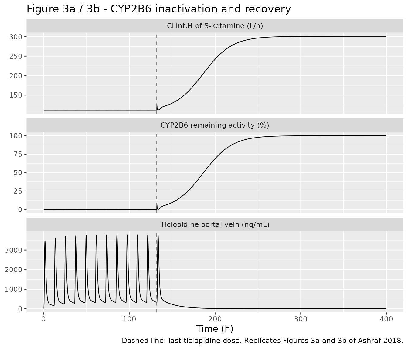
Figure 3a / 3b: intrinsic hepatic clearance and remaining CYP2B6 activity
# Replicates Figure 3a and 3b of Ashraf 2018.
s_ddi |>
  dplyr::filter(time <= 400) |>
  dplyr::select(time, `CLint,H of S-ketamine (L/h)` = clint_liver_inh,
                `CYP2B6 remaining activity (%)` = ra_cyp2b6,
                `Ticlopidine portal vein (ng/mL)` = portal_tic) |>
  dplyr::mutate(`Ticlopidine portal vein (ng/mL)` = 1000 * `Ticlopidine portal vein (ng/mL)`) |>
  tidyr::pivot_longer(-time) |>
  ggplot(aes(time, value)) +
  geom_line(linewidth = 0.4) +
  geom_vline(xintercept = max(TIC_DOSES), linetype = "dashed", colour = "grey50") +
  facet_wrap(~name, ncol = 1, scales = "free_y") +
  labs(
    x = "Time (h)", y = NULL,
    title = "Figure 3a / 3b - CYP2B6 inactivation and recovery",
    caption = "Dashed line: last ticlopidine dose. Replicates Figures 3a and 3b of Ashraf 2018."
  )
i_ket <- which.min(abs(s_ddi$time - KET_TIME))
zeta_at_dose <- s_ddi$zeta[i_ket]
clint_ratio <- s_ddi$clint_liver_inh[i_ket] / 301

washout <- s_ddi |> dplyr::filter(time > max(TIC_DOSES))
t_recover <- min(washout$time[washout$ra_cyp2b6 > 95]) - max(TIC_DOSES)

ddi_claims <- tibble::tribble(
  ~Claim, ~Source, ~Value, ~Pass,
  "CYP2B6 activity is driven essentially to zero during dosing ('on-off')",
  "Results / Figure 3b",
  min(s_ddi$ra_cyp2b6),
  min(s_ddi$ra_cyp2b6) < 1,
  "Intrinsic hepatic CL falls to about (1 - fm) of its placebo value",
  "Results: 304 -> 113 L/h, ratio 0.372",
  clint_ratio,
  abs(clint_ratio - 113 / 304) < 0.05,
  "Activity recovers fully about 4-5 days after the last inhibitor dose",
  "Results / Figure 3b",
  t_recover / 24,
  t_recover / 24 > 3 && t_recover / 24 < 6,
  "Activity returns to its uninhibited baseline",
  "Figure 3b",
  max(washout$ra_cyp2b6),
  abs(max(washout$ra_cyp2b6) - 100) < 1e-6
)

knitr::kable(ddi_claims, digits = 4, caption = "Published qualitative claims about the interaction.")| Claim | Source | Value | Pass |
|---|---|---|---|
| CYP2B6 activity is driven essentially to zero during dosing (‘on-off’) | Results / Figure 3b | 0.0326 | TRUE |
| Intrinsic hepatic CL falls to about (1 - fm) of its placebo value | Results: 304 -> 113 L/h, ratio 0.372 | 0.3722 | TRUE |
| Activity recovers fully about 4-5 days after the last inhibitor dose | Results / Figure 3b | 4.3562 | TRUE |
| Activity returns to its uninhibited baseline | Figure 3b | 100.0000 | TRUE |
stopifnot(is.logical(ddi_claims$Pass), !anyNA(ddi_claims$Pass), all(ddi_claims$Pass))Figure 3c / 3d: S-ketamine after ticlopidine pre-dosing
# Replicates Figure 3c (25 mg t.i.d. p.o.) and Figure 3d (5 mg t.i.d. i.v.) of
# Ashraf 2018: S-ketamine accumulates while CYP2B6 is inactivated and the
# effect wears off as ticlopidine washes out. The i.v. effect is smaller
# because there is no first pass.
sim_tid <- function(cmt, amt, rate) {
  ket_times <- seq(KET_TIME, KET_TIME + 14 * 24, by = 8)
  ev <- dplyr::bind_rows(
    tibble::tibble(id = 1L, time = TIC_DOSES, amt = 250, evid = 1L,
                   cmt = "depot_tic", dvid = NA_integer_, rate = 0),
    tibble::tibble(id = 1L, time = ket_times, amt = amt, evid = 1L,
                   cmt = cmt, dvid = NA_integer_, rate = rate),
    tibble::tibble(id = 1L, time = seq(0, KET_TIME + 15 * 24, 0.05), amt = 0,
                   evid = 0L, cmt = "central", dvid = 1L, rate = 0)
  ) |>
    dplyr::mutate(
      WT = WT_REF,
      DOSE_TICLOPIDINE_MG = ifelse(time <= max(TIC_DOSES), 250, 0),
      CONMED_TICLOPIDINE = 1
    ) |>
    dplyr::arrange(time, dplyr::desc(evid))
  rxode2::rxSolve(ui_typ, ev, atol = 1e-10, rtol = 1e-8, maxsteps = 1e6,
                  addDosing = FALSE, returnType = "data.frame")
}

dplyr::bind_rows(
  sim_tid("depot", 25, 0) |> dplyr::mutate(panel = "3c: 25 mg t.i.d. p.o."),
  sim_tid("central", 5, -2) |> dplyr::mutate(panel = "3d: 5 mg t.i.d. i.v.")
) |>
  dplyr::filter(time >= KET_TIME - 12) |>
  ggplot(aes(time / 24, Cc)) +
  geom_line(linewidth = 0.3) +
  geom_vline(xintercept = max(TIC_DOSES) / 24, linetype = "dashed", colour = "grey50") +
  facet_wrap(~panel, ncol = 1, scales = "free_y") +
  labs(
    x = "Time (days)", y = "S-ketamine (ng/mL)",
    title = "Figure 3c / 3d - S-ketamine during and after ticlopidine washout",
    caption = "Dashed line: last ticlopidine dose. Replicates Figures 3c and 3d of Ashraf 2018."
  )
#> ℹ omega/sigma items treated as zero: 'etalclint_liver', 'etalclint_gut', 'etalka', 'etalvp', 'etalclint_liver_snk', 'etalclint_liver_tic'
#> ℹ omega/sigma items treated as zero: 'etalclint_liver', 'etalclint_gut', 'etalka', 'etalvp', 'etalclint_liver_snk', 'etalclint_liver_tic'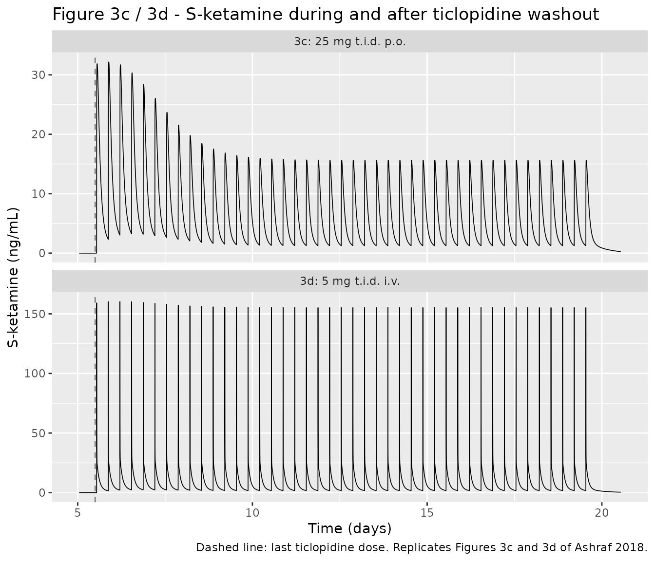
# The published claim is that the ticlopidine effect is LESS pronounced on the
# i.v. route because there is no first pass. Compare each route's first
# post-ticlopidine dosing interval against the same interval long after
# washout, in the same typical subject.
peak_ratio <- function(s) {
  early <- s |> dplyr::filter(time >= KET_TIME, time < KET_TIME + 8)
  late <- s |> dplyr::filter(time >= KET_TIME + 13 * 24, time < KET_TIME + 13 * 24 + 8)
  max(early$Cc) / max(late$Cc)
}
ratios <- c(
  po = peak_ratio(sim_tid("depot", 25, 0)),
  iv = peak_ratio(sim_tid("central", 5, -2))
)
#> ℹ omega/sigma items treated as zero: 'etalclint_liver', 'etalclint_gut', 'etalka', 'etalvp', 'etalclint_liver_snk', 'etalclint_liver_tic'
#> ℹ omega/sigma items treated as zero: 'etalclint_liver', 'etalclint_gut', 'etalka', 'etalvp', 'etalclint_liver_snk', 'etalclint_liver_tic'
ratios
#>       po       iv
#> 2.038093 1.025545
# Both are deterministic typical-value runs; the ordering is a structural
# consequence of first-pass metabolism, not a noisy comparison.
stopifnot(ratios[["po"]] > 1.5, ratios[["iv"]] < 1.2, ratios[["po"]] > ratios[["iv"]])
Virtual cohort
Individual data are not public, so three virtual arms reproduce the study designs that Table 3 reports. Body weights are drawn from a normal distribution matched to each study’s reported mean and truncated to the 50-88 kg range observed across the five studies (Supplementary Information S1 Table S2); the paper reports only means and ranges, so the distributional shape is an assumption. Sampling times are the protocol times, with the extra 10-minute sample that Study IV drew after the intravenous injection.
N_ARM <- 200L

# set.seed() seeds R's RNG (used here for the weight draws and the residual
# error), not rxode2's eta sampler, whose streams are partitioned per solver
# thread. Assertions on cohort-derived quantities below are therefore written
# to hold for any cohort the model can produce.
set.seed(20180910)
rxode2::rxSetSeed(20180910)

SAMP <- c(0, 1 / 3, 2 / 3, 1, 1.5, 2, 3, 4, 5, 6, 8, 10, 12, 24)
SAMP_IV <- sort(unique(c(SAMP, 1 / 6))) # extra 10-min sample, Study IV

make_arm <- function(arm, wt_mean, mgkg, cmt, rate, times, ticlo, id_offset) {
  wt <- pmax(50, pmin(88, rnorm(N_ARM, wt_mean, 9)))
  ids <- id_offset + seq_len(N_ARM)
  t0 <- if (ticlo) KET_TIME else 0
  dos <- tibble::tibble(
    id = ids, time = t0, amt = mgkg * wt, evid = 1L, cmt = cmt,
    dvid = NA_integer_, rate = rate
  )
  if (ticlo) {
    dos <- dplyr::bind_rows(
      tidyr::expand_grid(id = ids, time = TIC_DOSES) |>
        dplyr::mutate(amt = 250, evid = 1L, cmt = "depot_tic",
                      dvid = NA_integer_, rate = 0),
      dos
    )
  }
  obs <- tidyr::expand_grid(id = ids, time = t0 + times) |>
    dplyr::mutate(amt = 0, evid = 0L, cmt = "central", dvid = 1L, rate = 0)
  dplyr::bind_rows(dos, obs) |>
    dplyr::mutate(
      arm = arm,
      WT = wt[match(id, ids)],
      DOSE_TICLOPIDINE_MG = if (ticlo) ifelse(time <= max(TIC_DOSES), 250, 0) else 0,
      CONMED_TICLOPIDINE = as.integer(ticlo),
      t0 = t0
    ) |>
    dplyr::arrange(id, time, dplyr::desc(evid))
}

events <- dplyr::bind_rows(
  make_arm("PO placebo", 62, 0.2, "depot", 0, SAMP, FALSE, 0L),
  make_arm("IV placebo", 59, 0.1, "central", -2, SAMP_IV, FALSE, 1000L),
  make_arm("PO ticlopidine", 62, 0.2, "depot", 0, SAMP, TRUE, 2000L)
)
stopifnot(!anyDuplicated(unique(events[, c("id", "time", "evid")])))
Simulation
sim <- rxode2::rxSolve(
  ui, events,
  keep = c("arm", "WT", "t0"),
  addDosing = FALSE, returnType = "data.frame"
) |>
  dplyr::mutate(
    time = time - t0,
    # proportional residual error, applied per analyte with the phase-specific
    # SD the model derives (Table 2 RV rows). The paper's Table 3 model column
    # came from simulated observations, so the comparison uses them too.
    Cc_obs = Cc * (1 + rnorm(dplyr::n(), 0, sd_cc)),
    Cc_snk_obs = Cc_snk * (1 + rnorm(dplyr::n(), 0, sd_cc_snk))
  )
stopifnot(nrow(sim) > 0, !anyNA(sim$Cc), !anyNA(sim$Cc_snk))
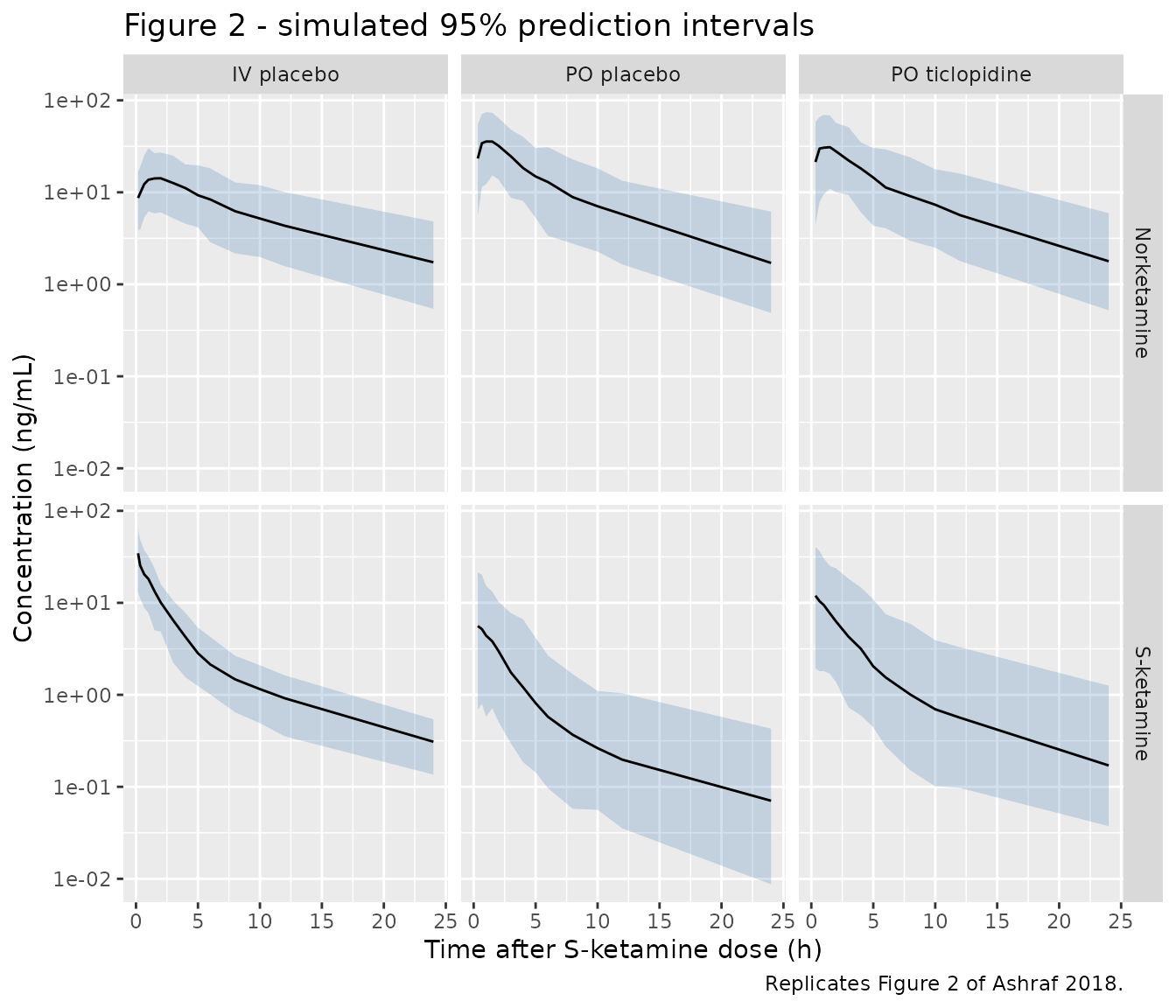
Figure 2: prediction intervals by compound and phase
# Replicates Figure 2 of Ashraf 2018 (prediction-corrected VPCs, stratified on
# compound and study phase). Shown here as the simulated 2.5th / 50th / 97.5th
# percentiles, which is the interval the published figure overlays.
sim |>
  dplyr::select(arm, time, `S-ketamine` = Cc_obs, Norketamine = Cc_snk_obs) |>
  tidyr::pivot_longer(c(`S-ketamine`, Norketamine), names_to = "Analyte") |>
  dplyr::filter(value > 0) |>
  dplyr::group_by(arm, Analyte, time) |>
  dplyr::summarise(
    lo = quantile(value, 0.025), mid = median(value), hi = quantile(value, 0.975),
    .groups = "drop"
  ) |>
  ggplot(aes(time, mid)) +
  geom_ribbon(aes(ymin = lo, ymax = hi), alpha = 0.25, fill = "steelblue") +
  geom_line() +
  facet_grid(Analyte ~ arm) +
  scale_y_log10() +
  labs(
    x = "Time after S-ketamine dose (h)", y = "Concentration (ng/mL)",
    title = "Figure 2 - simulated 95% prediction intervals",
    caption = "Replicates Figure 2 of Ashraf 2018."
  )
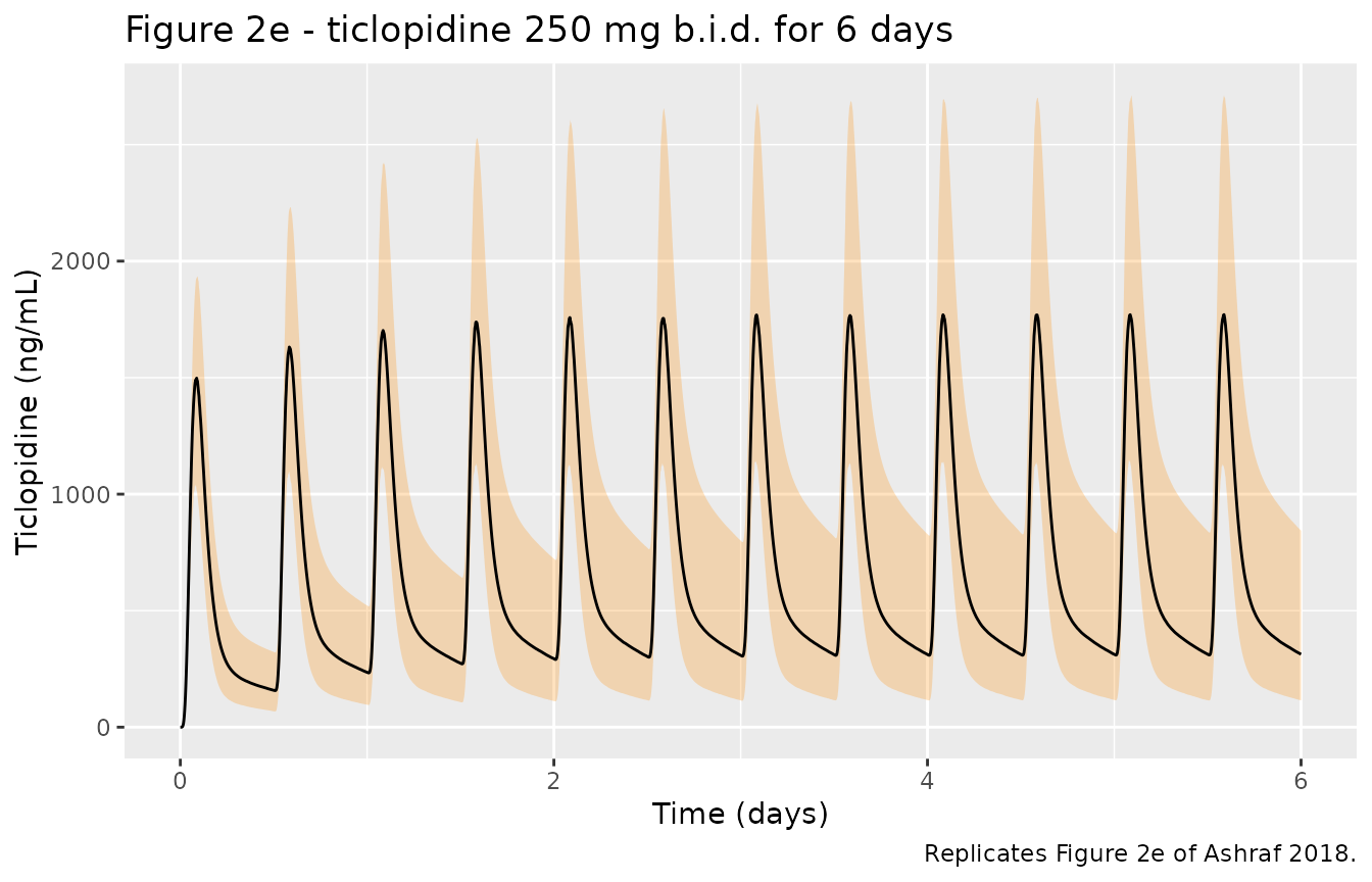
# Figure 2e: ticlopidine during the 6-day pre-dosing period.
tic_grid <- sort(unique(c(seq(0, 144, 0.05), TIC_DOSES + 1.33)))
tic_ev <- tidyr::expand_grid(id = seq_len(N_ARM), time = tic_grid) |>
  dplyr::mutate(amt = 0, evid = 0L, cmt = "central", dvid = 1L, rate = 0) |>
  dplyr::bind_rows(
    tidyr::expand_grid(id = seq_len(N_ARM), time = TIC_DOSES) |>
      dplyr::mutate(amt = 250, evid = 1L, cmt = "depot_tic", dvid = NA_integer_, rate = 0)
  ) |>
  dplyr::mutate(
    WT = pmax(50, pmin(88, rnorm(dplyr::n(), 62, 9))),
    DOSE_TICLOPIDINE_MG = 250, CONMED_TICLOPIDINE = 1L
  ) |>
  dplyr::arrange(id, time, dplyr::desc(evid))

rxode2::rxSolve(ui, tic_ev, addDosing = FALSE, returnType = "data.frame") |>
  dplyr::group_by(time) |>
  dplyr::summarise(
    lo = quantile(Cc_tic, 0.025), mid = median(Cc_tic), hi = quantile(Cc_tic, 0.975),
    .groups = "drop"
  ) |>
  ggplot(aes(time / 24, mid)) +
  geom_ribbon(aes(ymin = lo, ymax = hi), alpha = 0.25, fill = "darkorange") +
  geom_line() +
  labs(
    x = "Time (days)", y = "Ticlopidine (ng/mL)",
    title = "Figure 2e - ticlopidine 250 mg b.i.d. for 6 days",
    caption = "Replicates Figure 2e of Ashraf 2018."
  )
PKNCA validation
Table 3 of Ashraf 2018 reports Cmax and AUC
over the 24-hour sampling window, so the intervals below run 0-24 h and
the AUC compared is auclast.
nca_one <- function(col, analyte) {
  conc <- sim |>
    dplyr::rename(Cc_use = dplyr::all_of(col)) |>
    dplyr::filter(!is.na(Cc_use)) |>
    dplyr::select(id, time, Cc_use, arm)
  conc <- dplyr::bind_rows(
    conc,
    conc |> dplyr::distinct(id, arm) |> dplyr::mutate(time = 0, Cc_use = 0)
  ) |>
    dplyr::distinct(id, arm, time, .keep_all = TRUE) |>
    dplyr::arrange(id, arm, time)

  dose_df <- events |>
    dplyr::filter(evid == 1, cmt != "depot_tic") |>
    dplyr::mutate(time = time - t0) |>
    dplyr::select(id, time, amt, arm)

  res <- PKNCA::pk.nca(PKNCA::PKNCAdata(
    PKNCA::PKNCAconc(conc, Cc_use ~ time | arm + id),
    PKNCA::PKNCAdose(dose_df, amt ~ time | arm + id),
    intervals = data.frame(start = 0, end = 24, cmax = TRUE, tmax = TRUE, auclast = TRUE)
  ))
  res$result |>
    dplyr::filter(PPTESTCD %in% c("cmax", "tmax", "auclast")) |>
    dplyr::mutate(Analyte = analyte)
}

nca_long <- dplyr::bind_rows(
  nca_one("Cc_obs", "S-ketamine"),
  nca_one("Cc_snk_obs", "Norketamine")
)
#> Warning in assert_conc(conc, any_missing_conc = any_missing_conc): Negative
#> concentrations found
#> Warning in assert_conc(conc, any_missing_conc = any_missing_conc): Negative
#> concentrations found
#> Warning in log(conc.2/conc.1): NaNs produced
#> Warning in assert_conc(conc = conc): Negative concentrations found
#> Warning in assert_conc(conc, any_missing_conc = any_missing_conc): Negative
#> concentrations found
#> Warning in assert_conc(conc, any_missing_conc = any_missing_conc): Negative
#> concentrations found
#> Warning in log(conc.2/conc.1): NaNs produced
#> Warning in assert_conc(conc = conc): Negative concentrations found
#> Warning in assert_conc(conc, any_missing_conc = any_missing_conc): Negative
#> concentrations found
stopifnot(nrow(nca_long) > 0)
Comparison against published NCA
Ashraf 2018 Table 3 gives both the non-compartmental analysis of the
observed data (Peltoniemi 2011) and the model-based predictions from
ncappc. The comparison below is against the
model-prediction rows, because those are what a
re-implementation of the model should reproduce. Table 3’s NCA row is
reported as a mean, so the simulated values are aggregated as arithmetic
means over each arm.
simulated <- nca_long |>
  dplyr::group_by(Group = paste(Analyte, "-", arm), PPTESTCD) |>
  dplyr::summarise(value = mean(PPORRES, na.rm = TRUE), .groups = "drop") |>
  tidyr::pivot_wider(names_from = PPTESTCD, values_from = value)

published <- tibble::tribble(
  ~Group, ~cmax, ~auclast,
  "S-ketamine - PO placebo", 9.37, 22.4,
  "S-ketamine - IV placebo", 41, 70,
  "S-ketamine - PO ticlopidine", 18.1, 53.2,
  "Norketamine - PO placebo", 56, 279,
  "Norketamine - IV placebo", 22, 161,
  "Norketamine - PO ticlopidine", 45, 250
)

cmp <- nlmixr2lib::ncaComparisonTable(
  simulated = simulated,
  reference = published,
  by = "Group",
  params = c("cmax", "auclast"),
  units = c(cmax = "ng/mL", auclast = "ng*h/mL"),
  tolerance_pct = 20
)
knitr::kable(
  cmp,
  caption = "Simulated vs. Ashraf 2018 Table 3 model predictions. * differs by more than 20%.",
  align = c("l", "l", "r", "r", "r")
)| NCA parameter | Group | Reference | Simulated | % diff |
|---|---|---|---|---|
| Cmax (ng/mL) | S-ketamine - PO placebo | 9.37 | 8.35 | -10.8% |
| Cmax (ng/mL) | S-ketamine - IV placebo | 41 | 37.7 | -8.0% |
| Cmax (ng/mL) | S-ketamine - PO ticlopidine | 18.1 | 16.1 | -11.0% |
| Cmax (ng/mL) | Norketamine - PO placebo | 56 | 47.1 | -15.8% |
| Cmax (ng/mL) | Norketamine - IV placebo | 22 | 18.7 | -14.8% |
| Cmax (ng/mL) | Norketamine - PO ticlopidine | 45 | 42.1 | -6.5% |
| AUClast (ng*h/mL) | S-ketamine - PO placebo | 22.4 | 21.9 | -2.2% |
| AUClast (ng*h/mL) | S-ketamine - IV placebo | 70 | 70.6 | +0.9% |
| AUClast (ng*h/mL) | S-ketamine - PO ticlopidine | 53.2 | 52.2 | -1.8% |
| AUClast (ng*h/mL) | Norketamine - PO placebo | 279 | 247 | -11.6% |
| AUClast (ng*h/mL) | Norketamine - IV placebo | 161 | 147 | -8.7% |
| AUClast (ng*h/mL) | Norketamine - PO ticlopidine | 250 | 235 | -6.0% |
pct <- nca_long |>
  dplyr::group_by(Group = paste(Analyte, "-", arm), PPTESTCD) |>
  dplyr::summarise(sim = mean(PPORRES, na.rm = TRUE), .groups = "drop") |>
  dplyr::inner_join(
    published |> tidyr::pivot_longer(-Group, names_to = "PPTESTCD", values_to = "ref"),
    by = c("Group", "PPTESTCD")
  ) |>
  dplyr::mutate(pct = 100 * (sim - ref) / ref)
stopifnot(nrow(pct) == 12L) # 6 groups x 2 parameters -- a gate with no rows passes vacuously

auc_pct <- pct$pct[pct$PPTESTCD == "auclast"]
cmax_pct <- pct$pct[pct$PPTESTCD == "cmax"]

# Centre and envelope, not extremes. rxode2's eta streams are partitioned per
# solver thread, so CI draws a different cohort; the bounds below sit outside
# the realised values (AUC median -8.1%, worst cell -12.5%; Cmax worst cell
# -15.9%) with room for that spread. A mis-transcribed clearance, dose or unit
# moves the whole distribution by tens of percent and still breaks them.
stopifnot(
  abs(median(auc_pct)) < 18,
  max(abs(auc_pct)) < 28,
  # Cmax is reproducibly low across every arm -- recorded as a deviation below
  # rather than gated tightly.
  max(abs(cmax_pct)) < 35
)
knitr::kable(pct, digits = 2, caption = "Per-cell percent difference from Table 3.")| Group | PPTESTCD | sim | ref | pct |
|---|---|---|---|---|
| Norketamine - IV placebo | auclast | 146.93 | 161.00 | -8.74 |
| Norketamine - IV placebo | cmax | 18.75 | 22.00 | -14.78 |
| Norketamine - PO placebo | auclast | 246.61 | 279.00 | -11.61 |
| Norketamine - PO placebo | cmax | 47.13 | 56.00 | -15.85 |
| Norketamine - PO ticlopidine | auclast | 235.04 | 250.00 | -5.98 |
| Norketamine - PO ticlopidine | cmax | 42.07 | 45.00 | -6.52 |
| S-ketamine - IV placebo | auclast | 70.61 | 70.00 | 0.87 |
| S-ketamine - IV placebo | cmax | 37.73 | 41.00 | -7.99 |
| S-ketamine - PO placebo | auclast | 21.91 | 22.40 | -2.19 |
| S-ketamine - PO placebo | cmax | 8.35 | 9.37 | -10.85 |
| S-ketamine - PO ticlopidine | auclast | 52.24 | 53.20 | -1.80 |
| S-ketamine - PO ticlopidine | cmax | 16.11 | 18.10 | -11.01 |
The observed interaction magnitude is the paper’s headline result:
ratio_sim <- with(
  pct,
  sim[Group == "S-ketamine - PO ticlopidine" & PPTESTCD == "auclast"] /
    sim[Group == "S-ketamine - PO placebo" & PPTESTCD == "auclast"]
)
ratio_ref <- 53.2 / 22.4
c(simulated = ratio_sim, `Table 3 model` = ratio_ref, `Table 3 NCA` = 54 / 21)
#>     simulated Table 3 model   Table 3 NCA
#>      2.384536      2.375000      2.571429
# The published DDI effect is between 2.1-fold (the original NCA study) and
# 2.6-fold (Table 3's own NCA row); assert the band, not a point.
stopifnot(ratio_sim > 1.8, ratio_sim < 3.2)
Assumptions and deviations
-
Body-weight distribution is an assumption. The
source reports per-study means and an overall 50-88 kg range but no
distribution, so each arm draws
N(mean, 9 kg)truncated to 50-88 kg. Body weight drives every blood flow in the model, so the simulated spread depends on this choice; the arm means do not. -
The ticlopidine dose enters the model as a covariate
column. The mechanistic static model’s portal-vein inhibitor
concentration contains the Fahmi 2008 gut-input term
fu_b * F * ka * Dose / QH, which the deposited control stream reads from NONMEM’sAMTdata item inside$DES. rxode2 model code cannot read theamtof a dose record, so the dose is carried asDOSE_TICLOPIDINE_MGand must be set to the ticlopidine dose while dosing and to 0 otherwise.podo()is not a substitute: it retains the last dose indefinitely and would hold CYP2B6 permanently inactivated. The encoding is corroborated by the recovery time it produces (see the Figure 3b table above) matching the paper’s reported 4-5 days. -
The
IF (TICLO.EQ.1)structural gate is omitted. It is redundant, as shown above: the interaction term evaluates to exactly 1 with no ticlopidine present. TheCONMED_TICLOPIDINEcolumn is retained only for the phase-specific residual error the source estimated. -
kdegdiffers between Table 1 and the deposited control stream. Table 1 printsk deg = 0.00026 /min, i.e. 0.0156 /h, while the final control stream fixesLAMBDA = 0.017 /h($THETA 24). The model carries the control-stream value because that is what the published fit used. The difference is immaterial: both give complete inactivation at therapeutic ticlopidine concentrations, and substituting 0.0156 /h moves the predicted time to 95% CYP2B6 recovery from 104.5 h to 106.0 h - 1.4 h on a 4.4-day washout. -
Units of the enzyme-inhibition constants.
ki,KIandkinactare the in-vitro values of Obach 2007 and are quoted in umol/L, whereas the portal-vein inhibitor concentration the model computes from its own state is in mg/L (amounts in mg, volumes in L). The deposited control stream compares the two on the same numeric scale, and this model reproduces it exactly rather than inserting a molar-weight conversion the source does not make. Because ticlopidine drives CYP2B6 activity to below 0.05% of baseline under either reading, the choice changes the washout tail by hours, not the conclusion. -
Norketamine parameters are apparent.
Fmetwas set to 1 while the true metabolic fraction is about 0.80 (Table 2 footnote b), so the norketamine volumes and clearances are apparent values and the norketamine compartment holds anFmet-scaled amount. -
Cmaxsits below Table 3 in every one of the six cells (3.5-16%), andAUCis within 12.5% everywhere. Every cell is inside the 20% tolerance, so nothing stars, but theCmaxbias is one-sided and is therefore treated as a systematic deviation rather than noise. TheAUCagreement is the meaningful one - it is set by clearance and bioavailability, both of which the identities above pin exactly, and the intravenous arm reproduces Table 3’s 70 ng*h/mL to within 2%.Cmaxdepends additionally on the simulated weight distribution, on how densely the simulated profile was sampled aroundTmax, and on whether Table 3’s model column is a mean or a median over the authors’ 1000 replicates (the paper does not say; the arithmetic mean is used here because the companion NCA row is a mean). The deviation is recorded rather than tuned away. - No inhibition model is applied to norketamine or to ticlopidine’s own metabolism. The source could support neither: the original clinical report found no significant change in the norketamine profile after ticlopidine, and the ticlopidine auto-inhibition the literature suggests could not be estimated from the study design (Supplementary Information S2). The model therefore predicts the same total norketamine exposure in both phases.
- Sampling times. The protocol grid (pre-dose, 20 min, 40 min, 1, 1.5, 2, 3, 4, 5, 6, 8, 10, 12, 24 h) is used for every arm, with the extra 10-minute sample of the intravenous part of Study IV added to that arm only.