Donepezil oral and intranasal brain and blood PK in mice (Kaikousidis 2023)
Source:vignettes/articles/Kaikousidis_2023_donepezil_mouse.Rmd
Kaikousidis_2023_donepezil_mouse.RmdModel and source
- Citation: Kaikousidis C, Papakyriakopoulou P, Dokoumetzidis A, Valsami G. Donepezil Brain and Blood Pharmacokinetic Modeling after Nasal Film and Oral Solution Administration in Mice. Pharmaceutics. 2023;15(5):1409. doi:10.3390/pharmaceutics15051409
- Article (open access): https://doi.org/10.3390/pharmaceutics15051409
Kaikousidis et al. (2023) modelled serum and brain donepezil concentrations in mice after an oral solution and after a nasal film, in four stages. Each stage was fitted twice, once to the per-time-point mean concentrations and once to the raw concentrations of every animal pooled as one typical subject. The library carries the five models the paper reports with full parameter tables:
stems <- c(
  oral_mean = "Kaikousidis_2023_donepezil_oral_meandata_mouse",
  oral_raw = "Kaikousidis_2023_donepezil_oral_rawdata_mouse",
  in_mean = "Kaikousidis_2023_donepezil_intranasal_meandata_mouse",
  in_raw = "Kaikousidis_2023_donepezil_intranasal_rawdata_mouse",
  combined = "Kaikousidis_2023_donepezil_combined_mouse"
)
mods <- lapply(stems, function(s) rxode2::rxode2(readModelDb(s)))
tibble::tibble(
  Model = unname(stems),
  Source = c(
    "Table 2, Per Os - Mean Data", "Table 2, Per Os - Raw Data",
    "Table 3, IN - Mean Data", "Table 3, IN - Raw Data",
    "Table 4, Total Fit (Per Os + IN raw data)"
  )
) |>
knitr::kable()| Model | Source |
|---|---|
| Kaikousidis_2023_donepezil_oral_meandata_mouse | Table 2, Per Os - Mean Data |
| Kaikousidis_2023_donepezil_oral_rawdata_mouse | Table 2, Per Os - Raw Data |
| Kaikousidis_2023_donepezil_intranasal_meandata_mouse | Table 3, IN - Mean Data |
| Kaikousidis_2023_donepezil_intranasal_rawdata_mouse | Table 3, IN - Raw Data |
| Kaikousidis_2023_donepezil_combined_mouse | Table 4, Total Fit (Per Os + IN raw data) |
-
Oral models (Figure 2): first-order absorption from
a gut
depotinto blood (central), a blood-peripheral exchange, a one-way blood-to-brain transferk_central_brain(paperk23) that depletes blood, and a lumped brain eliminationkeff_brain(paperk30). The blood volume is fixed to 0.279 L from the paper’s preliminary blood-only fit (Table 1), which makes the brain volume identifiable. -
Intranasal models (Figure 4): the nasal-film dose
in
depot_nasalis split into a fractionP1absorbed into blood, a fraction(1 - P1) * P2absorbed directly into brain (both zero-order overTk0after a lagTlag), and the remainder(1 - P1) * (1 - P2), which reaches brain after a Savic transit chain (mean transit timeMtt, ratektr) and a first-order absorption step out ofdepot_brain(ka). There is no peripheral compartment.k23andk30are fixed to the oral values of the matching data representation. -
Combined model (Section 3.3): both sub-models
fitted jointly to the raw data, sharing the blood elimination,
blood-to-brain and brain elimination rate constants, with route-specific
apparent volumes and residual errors selected by
ROUTE_ORAL(1 = oral, 0 = nasal film). The authors present it as a check on the robustness of the staged fits and did not refine it further.
None of the models estimates between-animal variability: each is a typical-value model with residual error only.
Population
Eight-week-old C57BL/6J mice (Section 2.1) received either 0.2 mL of a 1.25 mg/mL donepezil solution by gastric gavage (0.25 mg, 10 mg/kg) or one nasal film containing 0.1 mg donepezil (4 mg/kg), which implies a body weight of about 25 g. Serum and perfused brain were sampled destructively at 5-360 min after the oral dose (n >= 5 per time point) and at 5-120 min after the nasal film (n = 3-5 per time point). Sex and the total number of animals are not reported. Concentrations below the LOQ (serum 0.043 ug/mL, brain 0.038 ug/mL) were set to LOQ/2 for fitting.
The same information is available programmatically, e.g.
readModelDb("Kaikousidis_2023_donepezil_combined_mouse")()$population.
Source trace
Every ini() value carries an in-file comment naming its
table row. The table below collects the typical values of all five
models, back-transformed from the packaged files, next to the paper
symbol and source table.
back_transform <- function(name, est) {
  dplyr::case_when(
    grepl("^logit", name) ~ 1 / (1 + exp(-est)),
    grepl("Sd", name) ~ est^2,
    grepl("^l", name) ~ exp(est),
    TRUE ~ est
  )
}
symbols <- tibble::tribble(
  ~name, ~symbol,
  "lka", "k12 (1/min)",
  "lkel", "k20 (1/min)",
  "lk_central_brain", "k23 (1/min)",
  "lk12", "k24 (1/min)",
  "lk21", "k42 (1/min)",
  "lkeff_brain", "k30 (1/min)",
  "lvc", "Vblood / V1 (L)",
  "lvc_oral", "Vblood, oral (L)",
  "lvc_intranasal", "Vblood_IN (L)",
  "lv_brain", "Vbrain / V2 (L)",
  "lv_brain_oral", "Vbrain_PO (L)",
  "lv_brain_intranasal", "Vbrain_IN (L)",
  "ltlag", "Tlag (min)",
  "ld1", "Tk0 (min)",
  "lmtt", "Mtt (min)",
  "lktr", "ktr (1/min)",
  "logitfrel", "P1",
  "logitfrel2", "P2",
  "lka_brain", "ka (1/min)",
  "propSd", "b1 (variance)",
  "propSd_Cbrain", "b2 (variance)",
  "addSd", "a1 (variance)",
  "addSd_Cbrain", "a2 (variance)",
  "addSd_oral", "a1 (variance)",
  "addSd_Cbrain_oral", "a2 (variance)",
  "addSd_intranasal", "a3 (variance)",
  "propSd_Cbrain_intranasal", "b1 (variance)"
)
trace <- dplyr::bind_rows(lapply(names(mods), function(m) {
  mods[[m]]$iniDf |>
    dplyr::filter(!is.na(ntheta)) |>
    dplyr::transmute(model = m, name, value = signif(back_transform(name, est), 3),
                     fixed = fix)
})) |>
  dplyr::mutate(value = ifelse(fixed, paste0(value, " (fixed)"), as.character(value))) |>
  dplyr::select(-fixed) |>
  tidyr::pivot_wider(names_from = model, values_from = value, values_fill = "") |>
  dplyr::left_join(symbols, by = "name") |>
  dplyr::relocate(symbol, .after = name)
stopifnot(!anyNA(trace$symbol))
trace |>
  dplyr::rename(
    "Parameter" = name, "Paper symbol" = symbol,
    "Oral, mean (Table 2)" = oral_mean, "Oral, raw (Table 2)" = oral_raw,
    "IN, mean (Table 3)" = in_mean, "IN, raw (Table 3)" = in_raw,
    "Combined (Table 4)" = combined
  ) |>
knitr::kable(caption = "Typical values on the paper's scale. Residual-error rows show the tabulated variance (the model stores its square root).")| Parameter | Paper symbol | Oral, mean (Table 2) | Oral, raw (Table 2) | IN, mean (Table 3) | IN, raw (Table 3) | Combined (Table 4) |
|---|---|---|---|---|---|---|
| lka | k12 (1/min) | 0.059 | 0.065 | 0.065 | ||
| lkel | k20 (1/min) | 0.012 | 0.017 | 0.046 | 0.05 | 0.039 |
| lk_central_brain | k23 (1/min) | 0.014 | 0.008 | 0.014 (fixed) | 0.008 (fixed) | 0.011 |
| lk12 | k24 (1/min) | 0.034 | 0.036 | 0.018 | ||
| lk21 | k42 (1/min) | 0.011 | 0.01 | 0.031 | ||
| lkeff_brain | k30 (1/min) | 0.325 | 0.369 | 0.325 (fixed) | 0.369 (fixed) | 0.276 |
| lvc | Vblood / V1 (L) | 0.279 (fixed) | 0.279 (fixed) | 0.021 | 0.027 | |
| lv_brain | Vbrain / V2 (L) | 0.018 | 0.009 | 0.005 | 0.003 | |
| propSd | b1 (variance) | 0.012 | ||||
| propSd_Cbrain | b2 (variance) | 0.062 | 0.043 | 0.238 | ||
| addSd | a1 (variance) | 0.016 | 0.016 | 0.082 | ||
| addSd_Cbrain | a2 (variance) | 0.004 | ||||
| ltlag | Tlag (min) | 4.06 | 3.72 | 3.59 | ||
| ld1 | Tk0 (min) | 11.3 | 11.6 | 11.4 | ||
| lmtt | Mtt (min) | 56 | 60.9 | 53.8 | ||
| lktr | ktr (1/min) | 0.171 | 0.183 | 0.205 | ||
| logitfrel | P1 | 0.543 | 0.683 | 0.557 | ||
| logitfrel2 | P2 | 0.3 | 0.276 | 0.306 | ||
| lka_brain | ka (1/min) | 0.173 | 0.566 | 0.127 | ||
| lvc_oral | Vblood, oral (L) | 0.279 (fixed) | ||||
| lv_brain_oral | Vbrain_PO (L) | 0.015 | ||||
| lvc_intranasal | Vblood_IN (L) | 0.024 | ||||
| lv_brain_intranasal | Vbrain_IN (L) | 0.005 | ||||
| addSd_oral | a1 (variance) | 0.017 | ||||
| addSd_Cbrain_oral | a2 (variance) | 0.004 | ||||
| addSd_intranasal | a3 (variance) | 0.084 | ||||
| propSd_Cbrain_intranasal | b1 (variance) | 0.236 |
| Equation | Source location |
|---|---|
| Oral structure: depot -> blood (k12), blood <-> peripheral (k24, k42), blood -> brain (k23), elimination from blood (k20) and brain (k30) | Figure 2; Section 3.1 |
Intranasal structure: depot -> blood and depot -> brain with
Tk0 and Tlag; depot -> transit chain ->
Abs -> brain (ktr, ka); blood -> brain
(k23); elimination k20, k30 |
Figure 4; Section 3.2 |
Dose split F2 = P2, F3 = (1 - P2) * P3,
F4 = (1 - P2) * (1 - P3)
|
Section 3.2 (printed as P1, P2 in Tables
3-4) |
Transit count N from ktr = (N + 1) / Mtt
(8.58 and 10.14 transit compartments) |
Section 3.2 |
| Residual error: proportional / additive per matrix and fit | Sections 3.1-3.3; Tables 2-4 |
The transit count is not a parameter of the files: it follows from
Mtt and ktr. The paper reports N = 8.58 (mean
data) and 10.14 (raw data). These equal ktr * Mtt - 1 for
both fits, i.e. the Savic relation ktr = (N + 1) / Mtt; the
formula as printed, (N - 1) / Mtt, would give 10.58 and
12.14.
ntr <- function(m) {
  th <- mods[[m]]$theta
  exp(th[["lmtt"]]) * exp(th[["lktr"]]) - 1
}
n_check <- c(in_mean = ntr("in_mean"), in_raw = ntr("in_raw"), combined = ntr("combined"))
round(n_check, 2)
#>  in_mean   in_raw combined
#>     8.58    10.14    10.03
stopifnot(abs(n_check[["in_mean"]] - 8.58) < 0.01, abs(n_check[["in_raw"]] - 10.14) < 0.01)
Simulation
All five models are deterministic at the typical value, so one
simulated mouse per route reproduces the paper’s fitted curves. Doses
are 0.25 mg into depot (oral) and 0.1 mg into
depot_nasal (nasal film). Each model has two observation
endpoints (Cc for serum, Cbrain for brain), so
the observation rows carry dvid = 1; rxode2 returns both
concentrations on every row.
make_events <- function(route, tend, by = 0.5) {
  dose <- if (route == "oral") {
    data.frame(id = 1L, time = 0, amt = 0.25, evid = 1L, cmt = "depot", dvid = NA_integer_)
  } else {
    data.frame(id = 1L, time = 0, amt = 0.1, evid = 1L, cmt = "depot_nasal", dvid = NA_integer_)
  }
  obs <- data.frame(id = 1L, time = seq(0, tend, by = by), amt = 0, evid = 0L,
                    cmt = NA_character_, dvid = 1L)
  ev <- rbind(dose, obs)
  ev$ROUTE_ORAL <- as.integer(route == "oral")
  ev
}
runs <- tibble::tribble(
  ~fit, ~model, ~route, ~tend, ~figure,
  "Oral, mean data", "oral_mean", "oral", 360, "Figure 3A (upper)",
  "Oral, raw data", "oral_raw", "oral", 360, "Figure 3A (lower)",
  "IN, mean data", "in_mean", "intranasal", 120, "Figure 5A (upper)",
  "IN, raw data", "in_raw", "intranasal", 120, "Figure 5A (lower)",
  "Combined, oral", "combined", "oral", 360, "Figure 6 (upper)",
  "Combined, IN", "combined", "intranasal", 120, "Figure 6 (lower)"
)
sim <- dplyr::bind_rows(lapply(seq_len(nrow(runs)), function(i) {
  ev <- make_events(runs$route[i], runs$tend[i])
  s <- as.data.frame(rxode2::rxSolve(mods[[runs$model[i]]], events = ev))
  s$fit <- runs$fit[i]
  s$route <- runs$route[i]
  s
})) |>
  dplyr::mutate(fit = factor(fit, levels = runs$fit))
# Integration noise only: states never go meaningfully negative.
stopifnot(all(sim$Cc >= -1e-6), all(sim$Cbrain >= -1e-6))
Checks of the intranasal input
The intranasal files write the lagged zero-order release and the
transit input as explicit functions of the nasal-film dose
(podo() / tad() of depot_nasal)
rather than with f(), alag() and
dur() on three dose records. With two endpoints, that form
(a lagged modelled-duration dose alongside the f() = 0
bolus that anchors the transit input) does not solve in rxode2 5.1.8
(“Duration is zero/negative”). The check below solves the intranasal
mean-data model against an independent single-endpoint formulation that
uses rxode2’s own lag, duration and bioavailability on three dose
records, and confirms mass balance with elimination switched off.
th <- mods$in_mean$theta
ref_mod <- rxode2::rxode2({
  ntr <- mtt * ktr - 1
  t_tr <- tad(depot_brain)
  transit_in <- 0
  if (t_tr > 0) transit_in <- (1 - p1) * (1 - p2) * exp(log(podo(depot_brain)) + log(ktr) + ntr * log(ktr * t_tr) - ktr * t_tr - lgamma(ntr + 1))
  d/dt(depot_brain) <- transit_in - ka_brain * depot_brain
  d/dt(central) <- -(kel + k_central_brain) * central
  d/dt(brain) <- ka_brain * depot_brain + k_central_brain * central - keff_brain * brain
  f(depot_brain) <- 0
  f(central) <- p1
  alag(central) <- tlag
  dur(central) <- d1
  f(brain) <- (1 - p1) * p2
  alag(brain) <- tlag
  dur(brain) <- d1
  Cc <- central / vc
  Cbrain <- brain / v_brain
})
ref_par <- c(
  mtt = exp(th[["lmtt"]]), ktr = exp(th[["lktr"]]), tlag = exp(th[["ltlag"]]),
  d1 = exp(th[["ld1"]]), p1 = plogis(th[["logitfrel"]]), p2 = plogis(th[["logitfrel2"]]),
  ka_brain = exp(th[["lka_brain"]]), kel = exp(th[["lkel"]]),
  k_central_brain = exp(th[["lk_central_brain"]]), keff_brain = exp(th[["lkeff_brain"]]),
  vc = exp(th[["lvc"]]), v_brain = exp(th[["lv_brain"]])
)
ref_ev <- rxode2::et(amt = 0.1, cmt = "central", rate = -2) |>
  rxode2::et(amt = 0.1, cmt = "brain", rate = -2) |>
  rxode2::et(amt = 0.1, cmt = "depot_brain") |>
  rxode2::et(seq(0, 120, by = 0.5))
ref <- as.data.frame(rxode2::rxSolve(ref_mod, params = ref_par, events = ref_ev))
pkg <- sim |> dplyr::filter(fit == "IN, mean data")
stopifnot(identical(ref$time, pkg$time))
rel_dev <- c(
  Cc = max(abs(pkg$Cc - ref$Cc)) / max(ref$Cc),
  Cbrain = max(abs(pkg$Cbrain - ref$Cbrain)) / max(ref$Cbrain)
)
signif(rel_dev, 2)
#>      Cc  Cbrain
#> 2.3e-06 8.1e-06
# Two independent ODE solutions at the default tolerances (rtol 1e-6);
# the observed agreement is about 1e-6.
stopifnot(all(rel_dev < 1e-3))

# Mass balance: with blood and brain elimination switched off the whole
# 0.1 mg dose ends up in the model states.
mb <- as.data.frame(rxode2::rxSolve(
  mods$in_mean, events = make_events("intranasal", 600),
  params = c(lkel = -40, lkeff_brain = -40)
))
mass_end <- with(mb[nrow(mb), ], depot_nasal + depot_brain + central + brain)
mass_end
#> [1] 0.1
stopifnot(abs(mass_end / 0.1 - 1) < 1e-4)
The dose split implied by the fractions, compared with the Discussion’s summary (direct-to-blood about half the dose, delayed transit fraction 25-30%):
split <- dplyr::bind_rows(lapply(c("in_mean", "in_raw", "combined"), function(m) {
  th <- mods[[m]]$theta
  p1 <- plogis(th[["logitfrel"]])
  p2 <- plogis(th[["logitfrel2"]])
  tibble::tibble(model = m, blood = p1, direct_brain = (1 - p1) * p2,
                 transit_brain = (1 - p1) * (1 - p2))
}))
split |>
  dplyr::mutate(dplyr::across(-model, \(x) round(x, 3))) |>
  dplyr::rename("Model" = model, "Direct to blood" = blood,
                "Direct to brain" = direct_brain, "Transit to brain" = transit_brain) |>
knitr::kable()| Model | Direct to blood | Direct to brain | Transit to brain |
|---|---|---|---|
| in_mean | 0.543 | 0.137 | 0.320 |
| in_raw | 0.683 | 0.087 | 0.230 |
| combined | 0.557 | 0.136 | 0.307 |
Replicate published figures
The points are values the maintainers read off the fitted curves in the paper’s figures (peaks, the intranasal brain trough between the two peaks, and selected late times); the lines are the packaged models.
fig_reads <- tibble::tribble(
  ~fit, ~matrix, ~time, ~value,
  "Oral, mean data", "Blood", 17, 0.355,
  "Oral, mean data", "Brain", 20, 0.215,
  "Oral, mean data", "Blood", 120, 0.065,
  "Oral, mean data", "Brain", 120, 0.045,
  "Oral, mean data", "Blood", 360, 0.022,
  "Oral, raw data", "Blood", 17, 0.355,
  "Oral, raw data", "Brain", 20, 0.215,
  "IN, mean data", "Blood", 15, 1.85,
  "IN, mean data", "Brain", 15, 1.03,
  "IN, mean data", "Brain", 30, 0.27,
  "IN, mean data", "Brain", 60, 0.49,
  "IN, raw data", "Blood", 15, 1.80,
  "IN, raw data", "Brain", 15, 0.97,
  "IN, raw data", "Brain", 30, 0.25,
  "IN, raw data", "Brain", 60, 0.50,
  "Combined, oral", "Blood", 17, 0.355,
  "Combined, oral", "Brain", 20, 0.23,
  "Combined, IN", "Blood", 15, 1.75,
  "Combined, IN", "Brain", 15, 1.00,
  "Combined, IN", "Brain", 60, 0.50
) |>
  dplyr::mutate(fit = factor(fit, levels = runs$fit))

sim_long <- sim |>
  dplyr::select(fit, time, Blood = Cc, Brain = Cbrain) |>
  tidyr::pivot_longer(c(Blood, Brain), names_to = "matrix", values_to = "conc")
ggplot(sim_long, aes(time, conc, colour = matrix)) +
  geom_line(linewidth = 0.8) +
  geom_point(data = fig_reads, aes(time, value), shape = 21, fill = "white", size = 2) +
  facet_wrap(~fit, ncol = 2, scales = "free") +
  scale_colour_manual(values = c(Blood = "#1f77b4", Brain = "#2ca02c")) +
  labs(x = "Time (min)", y = "Donepezil (ug/mL)", colour = NULL,
       caption = "Replicates Figures 3A, 5A and 6 of Kaikousidis 2023 (fitted curves).") +
  theme_bw() +
  theme(legend.position = "bottom")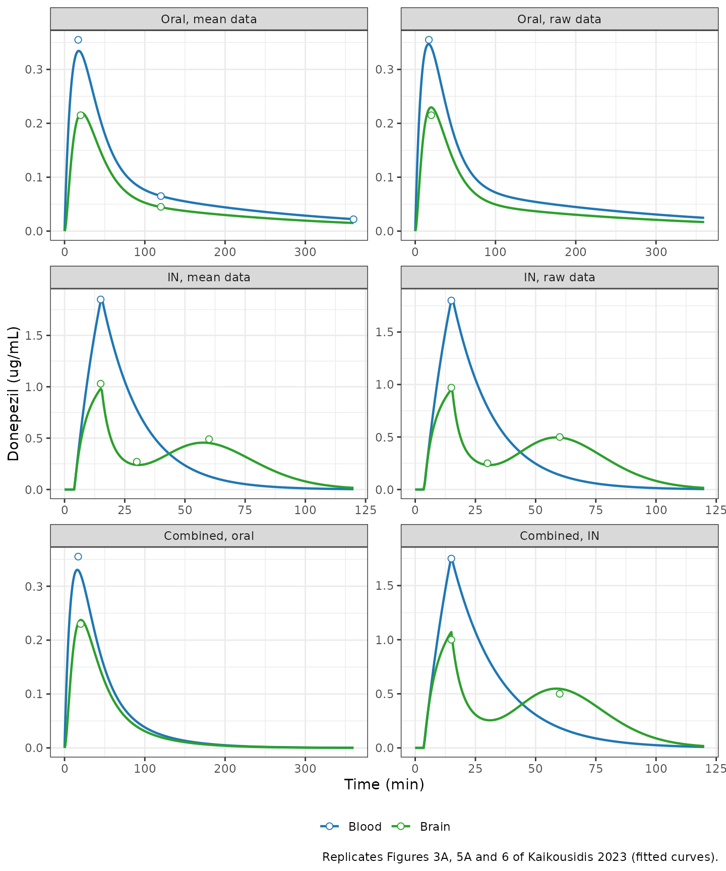
fig_check <- fig_reads |>
  dplyr::left_join(sim_long, by = c("fit", "matrix", "time")) |>
  dplyr::mutate(pct_diff = 100 * (conc / value - 1))
fig_check |>
  dplyr::mutate(conc = signif(conc, 3), pct_diff = round(pct_diff, 1)) |>
  dplyr::rename("Fit" = fit, "Matrix" = matrix, "Time (min)" = time,
                "Read from figure (ug/mL)" = value, "Model (ug/mL)" = conc,
                "% diff" = pct_diff) |>
knitr::kable()| Fit | Matrix | Time (min) | Read from figure (ug/mL) | Model (ug/mL) | % diff |
|---|---|---|---|---|---|
| Oral, mean data | Blood | 17 | 0.355 | 0.3340 | -5.9 |
| Oral, mean data | Brain | 20 | 0.215 | 0.2190 | 1.7 |
| Oral, mean data | Blood | 120 | 0.065 | 0.0651 | 0.2 |
| Oral, mean data | Brain | 120 | 0.045 | 0.0444 | -1.2 |
| Oral, mean data | Blood | 360 | 0.022 | 0.0222 | 0.9 |
| Oral, raw data | Blood | 17 | 0.355 | 0.3470 | -2.3 |
| Oral, raw data | Brain | 20 | 0.215 | 0.2300 | 6.8 |
| IN, mean data | Blood | 15 | 1.850 | 1.8400 | -0.8 |
| IN, mean data | Brain | 15 | 1.030 | 0.9810 | -4.7 |
| IN, mean data | Brain | 30 | 0.270 | 0.2390 | -11.4 |
| IN, mean data | Brain | 60 | 0.490 | 0.4530 | -7.6 |
| IN, raw data | Blood | 15 | 1.800 | 1.8100 | 0.3 |
| IN, raw data | Brain | 15 | 0.970 | 0.9540 | -1.6 |
| IN, raw data | Brain | 30 | 0.250 | 0.2330 | -6.7 |
| IN, raw data | Brain | 60 | 0.500 | 0.4950 | -1.0 |
| Combined, oral | Blood | 17 | 0.355 | 0.3300 | -7.1 |
| Combined, oral | Brain | 20 | 0.230 | 0.2370 | 3.2 |
| Combined, IN | Blood | 15 | 1.750 | 1.7700 | 1.0 |
| Combined, IN | Brain | 15 | 1.000 | 1.0700 | 7.1 |
| Combined, IN | Brain | 60 | 0.500 | 0.5460 | 9.3 |
# Typical-value solves, no random draws: every model point sits within 12%
# of the curve read off the paper's figure (largest 11%, the shallow brain
# trough at 30 min). Fixing the raw-data intranasal fit's k23/k30 to the
# mean-data oral values instead moves its first brain peak by +34%.
stopifnot(!anyNA(fig_check$conc), all(abs(fig_check$pct_diff) < 15))
The intranasal brain curve shows the paper’s double peak: the direct
nose-to-brain input peaks at the end of the zero-order window
(Tlag + Tk0, about 15 min) and the transit-delayed input
produces the second peak near 60 min.
second_peak <- sim |>
  dplyr::filter(route == "intranasal", time > 30) |>
  dplyr::group_by(fit) |>
  dplyr::summarise(t_second_peak = time[which.max(Cbrain)], .groups = "drop")
second_peak
#> # A tibble: 3 × 2
#>   fit           t_second_peak
#>   <fct>                 <dbl>
#> 1 IN, mean data          57.5
#> 2 IN, raw data           58.5
#> 3 Combined, IN           58.5
stopifnot(all(second_peak$t_second_peak > 45 & second_peak$t_second_peak < 75))
PKNCA validation
Non-compartmental analysis of the typical curves, one PKNCA block per matrix, grouped by fit. The oral curves end at the last oral sample (360 min) and the intranasal curves at the last intranasal sample (120 min).
run_nca <- function(conc_col) {
  conc <- sim |>
    dplyr::filter(!is.na(.data[[conc_col]])) |>
    dplyr::transmute(id = 1L, fit = as.character(fit), time, conc = pmax(.data[[conc_col]], 0))
  stopifnot(all(conc |> dplyr::group_by(fit) |> dplyr::summarise(t0 = min(time)) |> dplyr::pull(t0) == 0))
  dose <- runs |>
    dplyr::transmute(id = 1L, fit, time = 0, amt = ifelse(route == "oral", 0.25, 0.1))
  conc_obj <- PKNCA::PKNCAconc(conc, conc ~ time | fit + id)
  dose_obj <- PKNCA::PKNCAdose(dose, amt ~ time | fit + id)
  intervals <- data.frame(start = 0, end = Inf, cmax = TRUE, tmax = TRUE, auclast = TRUE)
  PKNCA::pk.nca(PKNCA::PKNCAdata(conc_obj, dose_obj, intervals = intervals))
}
nca_blood <- run_nca("Cc")
nca_brain <- run_nca("Cbrain")
nca_tab <- dplyr::bind_rows(
  as.data.frame(nca_blood) |> dplyr::mutate(matrix = "Blood"),
  as.data.frame(nca_brain) |> dplyr::mutate(matrix = "Brain")
) |>
  dplyr::select(fit, matrix, PPTESTCD, PPORRES) |>
  tidyr::pivot_wider(names_from = PPTESTCD, values_from = PPORRES) |>
  dplyr::mutate(fit = factor(fit, levels = runs$fit)) |>
  dplyr::arrange(matrix, fit)
nca_tab |>
  dplyr::mutate(cmax = signif(cmax, 3), auclast = signif(auclast, 3)) |>
  dplyr::rename("Fit" = fit, "Matrix" = matrix, "Cmax (ug/mL)" = cmax,
                "Tmax (min)" = tmax, "AUClast (ug*min/mL)" = auclast) |>
knitr::kable()| Fit | Matrix | AUClast (ug*min/mL) | Cmax (ug/mL) | Tmax (min) |
|---|---|---|---|---|
| Oral, mean data | Blood | 29.3 | 0.334 | 17.5 |
| Oral, raw data | Blood | 29.2 | 0.347 | 16.5 |
| IN, mean data | Blood | 43.0 | 1.860 | 15.5 |
| IN, raw data | Blood | 43.5 | 1.820 | 15.5 |
| Combined, oral | Blood | 17.9 | 0.330 | 16.0 |
| Combined, IN | Blood | 46.2 | 1.770 | 15.0 |
| Oral, mean data | Brain | 19.5 | 0.219 | 21.5 |
| Oral, raw data | Brain | 19.6 | 0.230 | 20.0 |
| IN, mean data | Brain | 35.7 | 0.981 | 15.0 |
| IN, raw data | Brain | 37.0 | 0.954 | 15.0 |
| Combined, oral | Brain | 13.3 | 0.237 | 20.5 |
| Combined, IN | Brain | 40.8 | 1.070 | 15.0 |
Comparison against published values
The Discussion reports that after the nasal film both serum and brain reach their maximum at the 15-min sampling time:
in_fits <- c("IN, mean data", "IN, raw data", "Combined, IN")
reference <- data.frame(fit = in_fits, tmax = 15)
cmp <- dplyr::bind_rows(
  nlmixr2lib::ncaComparisonTable(
    simulated = as.data.frame(nca_blood) |> dplyr::filter(fit %in% in_fits),
    reference = reference, by = "fit", params = "tmax", units = c(tmax = "min")
  ) |> dplyr::mutate(Matrix = "Blood", .before = 2),
  nlmixr2lib::ncaComparisonTable(
    simulated = as.data.frame(nca_brain) |> dplyr::filter(fit %in% in_fits),
    reference = reference, by = "fit", params = "tmax", units = c(tmax = "min")
  ) |> dplyr::mutate(Matrix = "Brain", .before = 2)
)
knitr::kable(cmp, caption = "Simulated vs. published Tmax after the nasal film. * differs from reference by >20%.")| NCA parameter | Matrix | fit | Reference | Simulated | % diff |
|---|---|---|---|---|---|
| Tmax (min) | Blood | IN, mean data | 15 | 15.5 | +3.3% |
| Tmax (min) | Blood | IN, raw data | 15 | 15.5 | +3.3% |
| Tmax (min) | Blood | Combined, IN | 15 | 15 | +0.0% |
| Tmax (min) | Brain | IN, mean data | 15 | 15 | +0.0% |
| Tmax (min) | Brain | IN, raw data | 15 | 15 | +0.0% |
| Tmax (min) | Brain | Combined, IN | 15 | 15 | +0.0% |
tmax_in <- nca_tab |> dplyr::filter(fit %in% in_fits) |> dplyr::pull(tmax)
stopifnot(all(abs(tmax_in - 15) <= 1.5))
The Discussion also quotes intranasal-to-oral ratios of Cmax and AUC from the non-compartmental analysis of the observed data in the authors’ earlier study (Papakyriakopoulou et al. 2023): Cmax 3.9-fold (blood) and 5.7-fold (brain) higher, and AUC 1.4-fold (blood) and 3.1-fold (brain) higher after the nasal film, at a 2.5-fold lower dose. The model-based ratios are shown for comparison; they are not a gate, because that analysis is of the observed mean data rather than of these fitted curves, and the AUC interval of that analysis is not stated.
ratio <- function(oral_fit, in_fit) {
  nca_tab |>
    dplyr::filter(fit %in% c(oral_fit, in_fit)) |>
    dplyr::mutate(route = ifelse(fit == in_fit, "in", "oral")) |>
    dplyr::select(matrix, route, cmax, auclast) |>
    tidyr::pivot_wider(names_from = route, values_from = c(cmax, auclast)) |>
    dplyr::transmute(matrix, cmax_ratio = cmax_in / cmax_oral,
                     auclast_ratio = auclast_in / auclast_oral)
}
ratios <- dplyr::bind_rows(
  ratio("Oral, mean data", "IN, mean data") |> dplyr::mutate(source = "Mean-data models"),
  ratio("Oral, raw data", "IN, raw data") |> dplyr::mutate(source = "Raw-data models"),
  ratio("Combined, oral", "Combined, IN") |> dplyr::mutate(source = "Combined model"),
  tibble::tibble(matrix = c("Blood", "Brain"), cmax_ratio = c(3.9, 5.7),
                 auclast_ratio = c(1.4, 3.1), source = "Reported (observed NCA)")
)
ratios |>
  dplyr::mutate(dplyr::across(c(cmax_ratio, auclast_ratio), \(x) round(x, 1))) |>
  dplyr::arrange(matrix) |>
  dplyr::rename("Matrix" = matrix, "Cmax IN / oral" = cmax_ratio,
                "AUC IN / oral" = auclast_ratio, "Source" = source) |>
knitr::kable()| Matrix | Cmax IN / oral | AUC IN / oral | Source |
|---|---|---|---|
| Blood | 5.6 | 1.5 | Mean-data models |
| Blood | 5.3 | 1.5 | Raw-data models |
| Blood | 5.3 | 2.6 | Combined model |
| Blood | 3.9 | 1.4 | Reported (observed NCA) |
| Brain | 4.5 | 1.8 | Mean-data models |
| Brain | 4.2 | 1.9 | Raw-data models |
| Brain | 4.5 | 3.1 | Combined model |
| Brain | 5.7 | 3.1 | Reported (observed NCA) |
The model-based brain Cmax ratio (4.2-4.5) is lower than the reported 5.7-fold, and the blood Cmax ratio (5.3-5.6) is higher than the reported 3.9-fold. The model-based AUC ratios over each route’s own sampling window match the reported blood ratio for the separate fits (1.5 vs 1.4) and the reported brain ratio for the combined fit (3.1 vs 3.1). The separate fits give 1.8-1.9 for brain, and the combined fit gives 2.6 for blood, because its faster blood elimination shortens the oral serum curve. The paper does not give the AUC interval or say whether the ratios are dose-normalised, so these differences cannot be attributed to the model.
Assumptions and deviations
-
Residual-error scale. Tables 2-4 print the
residual-error parameters (
a1,a2,a3,b1,b2) without saying whether they are variances or standard deviations. The maintainers read them as NONMEM variances and store their square roots. Read as standard deviations, the oral raw-data additive error on serum (0.016 ug/mL) would put 90% of observations within +/-0.026 ug/mL of a 0.33 ug/mL peak. The raw serum data in Figure 3A (lower) span about 0.13-0.72 ug/mL around that peak, which matches the variance reading (SD 0.126 ug/mL, 90% interval about 0.12-0.54 ug/mL). The intranasal raw serum data (Figure 5A, lower: about 0.2-1.3 ug/mL at 30 min) likewise fit an SD of sqrt(0.082) = 0.29 ug/mL better than 0.082 ug/mL. The proportional rows are read on the same scale. -
Mislabelled table blocks. Table 3 prints its
residual-error block under “Per Os” headings, although the block sits in
the intranasal table and has the intranasal structure the text describes
(additive serum, proportional brain). Table 4’s footnote labels
b1/b2as intranasal blood / brain, but the table rows area1,a2,a3,b1, and the text says the intranasal blood error is additive. The rows are assigned by the text:a3is the intranasal serum additive error andb1the intranasal brain proportional error, matching the separate intranasal raw-data fit (0.084 vs 0.082 and 0.236 vs 0.238). -
Fraction notation. Section 3.2 writes the dose
split with
P2(blood) andP3(direct brain), while Tables 3-4 print them asP1andP2, and the Table 4 footnote callsP2the “fraction of dose absorbed in brain”. The packaged models follow the printed equation (P2is the share of the non-blood dose, not of the whole dose); where the paper’s equation and its labels disagree, the maintainers follow the equation. The Discussion’s figures of “25-30%” for the transit fraction and “20-25%” for the olfactory fraction match neither reading exactly. -
Rate-constant labels in Section 3.2. The text says
that “the blood-to-brain transfer (k23) and the brain elimination (k20)
were fixed … while the blood elimination (k30) was taken as a prior”.
Figure 4 and the Table 3 footnote name k20 as blood elimination
(estimated, 0.046 / 0.05 1/min) and k30 as brain elimination, so
k23andk30are the fixed pair. The text does not say which oral fit supplied them. Fixing them to the matching data representation (mean to mean, raw to raw) reproduces Figure 5. The other pairing moves the raw-data intranasal brain peak from 0.95 to 1.28 ug/mL (Figure 5 about 0.97). - Oral blood volume in the combined fit. Table 4 does not list the oral blood volume. It is taken as the fixed 0.279 L of the oral sub-model (Section 3.1), which reproduces the oral panels of Figure 6.
- No peripheral compartment after intranasal dosing in the combined fit. Section 3.3 joins “the two previous individual models”, and the intranasal model (Figure 4) has no peripheral compartment. With the oral peripheral exchange also applied to intranasal dosing, the combined model’s intranasal serum peak would drop from 1.77 to 1.63 ug/mL and the curve would keep a slow tail (0.05 ug/mL at 120 min) that Figure 6 does not show.
-
Transit relation. The printed
ktr = (N - 1) / Mttis read asktr = (N + 1) / Mtt, the only form that reproduces the reported N = 8.58 and 10.14 (checked above). -
Lag time and duration in the combined fit. Table 4
reports
TlagandTk0with relative standard errors of 0.11% and 0.06%. They are estimates, not fixed values, and are packaged as estimated. -
Single nasal-film dose. The explicit intranasal
input is keyed on the most recent
depot_nasaldose (podo()/tad()). The models are valid for the single doses the paper studied, or for doses spaced beyond the transit chain (about 3 xMtt). - Preliminary blood-only fit not packaged. The two-compartment fit to the oral serum data (Table 1) is the first stage of the oral model and only serves to fix the blood volume. It is not packaged as a separate model.
- No correction notice for the article was found (search on 2026-10-26).