Empagliflozin (Jiang 2024)
Source:vignettes/articles/Jiang_2024_empagliflozin.Rmd
Jiang_2024_empagliflozin.RmdModel and source
mod <- rxode2::rxode2(readModelDb("Jiang_2024_empagliflozin"))
#> ℹ parameter labels from comments will be replaced by 'label()'
#> Warning: some etas defaulted to non-mu referenced, possible parsing error: etaiov_ktr_1, etaiov_ktr_2, etaiov_mtt_1, etaiov_mtt_2, etaiov_ka_1, etaiov_ka_2, etaiov_cl_1, etaiov_cl_2
#> as a work-around try putting the mu-referenced expression on a simple line- Citation: Jiang X, Yu KS, Nam DH, Oh J. A Population Pharmacokinetic Study to Compare a Novel Empagliflozin L-Proline Formulation with Its Conventional Formulation in Healthy Subjects. Pharmaceuticals (Basel). 2024 Apr 18;17(4):522. doi:10.3390/ph17040522.
- Article: https://doi.org/10.3390/ph17040522
- PubMed Central: https://www.ncbi.nlm.nih.gov/pmc/articles/PMC11054906/
Jiang 2024 pooled two randomized, open-label, two-period, two-sequence crossover phase 1 studies to ask a single question: does formulating empagliflozin as an L-proline cocrystal (CKD-370) change its pharmacokinetics relative to the conventional formulation? The answer reported by the paper is no. Formulation (“treatment”) was screened as a covariate and was not retained, so the packaged model is deliberately formulation-agnostic and predicts identical profiles for both products. This vignette asserts that invariance numerically rather than merely restating it.
Population
54 healthy Korean adults (27 per study) contributed 1832 plasma empagliflozin concentrations: 864 from Study A (NCT03849495; 25 mg empagliflozin L-proline vs 25 mg conventional empagliflozin) and 968 from Study B (NCT03848637; 5 mg/1000 mg empagliflozin L-proline/metformin vs 5 mg/1000 mg empagliflozin/metformin fixed-dose combinations). Pooled baseline characteristics (Table 1): median age 27.5 years [20-50], median weight 72.1 kg [55.6-83.4] (mean 69.69 +/- 7.82), median BMI 24.1 kg/m^2 [19.5-26.9], median MDRD eGFR 112.35 mL/min/1.73 m^2 [74.2-143.9]. 12 of 54 subjects (22.2%) were female. Eligibility required age 19-50 years and BMI 18-27 kg/m^2, so the cohort is narrow: healthy, young, normal-weight, normal-renal-function, and entirely Korean. The paper lists the healthy-subject-only composition, the single ethnicity, and the absence of an external validation dataset as its three stated limitations.
The same information is available programmatically via
readModelDb("Jiang_2024_empagliflozin")()$population.
Source trace
Every ini() entry carries an in-file comment naming its
source location in
inst/modeldb/specificDrugs/Jiang_2024_empagliflozin.R. They
are collected here for review. All fixed-effect and random-effect values
come from Jiang 2024 Table 2, “Estimates of population pharmacokinetics
parameters”; every one is corroborated by the bootstrap median reported
in the same row (1000 resamples).
| Equation / parameter | Value | Source location |
|---|---|---|
lktr (Ktr) |
9.19 1/h | Table 2, Fixed effects (RSE 12.4%; bootstrap 8.94 [6.766-11.728]) |
lmtt (Mtt) |
0.63 h | Table 2, Fixed effects (RSE 4.26%; bootstrap 0.64 [0.526-0.725]) |
lka (Ka) |
0.26 1/h | Table 2, Fixed effects (RSE 3.42%; bootstrap 0.25 [0.23-0.275]) |
lcl (CL/F) |
8.21 L/h | Table 2, Fixed effects (RSE 1.78%; bootstrap 8.21 [7.945-8.465]) |
lvc (V1/F, central) |
0.6 L | Table 2, Fixed effects (RSE 6.67%; bootstrap 0.64 [0-1.889]) |
lvp (V2/F, peripheral) |
44.6 L | Table 2, Fixed effects (RSE 2.51%; bootstrap 43.93 [41.255-47.171]) |
lq (Q/F) |
4.92 L/h | Table 2, Fixed effects (RSE 5.09%; bootstrap 4.66 [3.979-5.456]) |
e_wt_cl (beta_CL_logWT) |
0.64 | Table 2, Fixed effects (RSE 24.5%; bootstrap 0.64 [0.366-0.926]) |
e_wt_vp (beta_V2_logWT) |
0.57 | Table 2, Fixed effects (RSE 30.3%; bootstrap 0.54 [0.221-0.851]) |
etalka (omega_Ka) |
0.17 SD -> var 0.0289 | Table 2, IIV block (17.12% CV, RSE 10.8%) |
etalcl (omega_CL) |
0.12 SD -> var 0.0144 | Table 2, IIV block (12.04% CV, RSE 10.9%) |
etalvp (omega_V2) |
0.13 SD -> var 0.0169 | Table 2, IIV block (13.06% CV, RSE 12.0%) |
etaiov_ktr_* (gamma_Ktr) |
1.17 SD -> var 1.3689 | Table 2, IOV block (171.20% CV, RSE 7.43%) |
etaiov_mtt_* (gamma_Mtt) |
0.42 SD -> var 0.1764 | Table 2, IOV block (43.92% CV, RSE 7.15%) |
etaiov_ka_* (gamma_Ka) |
0.029 SD -> var 0.000841 | Table 2, IOV block (2.90% CV, RSE 34.3%) |
etaiov_cl_* (gamma_CL) |
0.043 SD -> var 0.001849 | Table 2, IOV block (4.30% CV, RSE 16.7%) |
propSd (b) |
0.16 | Table 2, Residual variability (RSE 2.01%; bootstrap 0.16 [0.141-0.175]) |
| Structural model: 2-compartment + transit absorption | n/a | Results 2.2 and Figure 1 |
N = Ktr * Mtt - 1 (transit chain length) |
4.79 | Formula (1), Mtt = (n+1)/Ktr; value quoted in Results
2.3 |
| Weight on CL and V2, log-transformed | n/a | Results 2.3; coefficients in Table 2 |
| Proportional residual error | n/a | Results 2.2 (“A proportional error model was found to best describe the residuals”) |
| Log-normal IIV / IOV, exponential random effects | n/a | Methods 4.3, Formulas (2) and (3) |
| IOV assigned to Ktr, Mtt, Ka, CL; IIV to Ka, CL, V2 | n/a | Results 2.3 |
Reading the random-effect column correctly
Table 2’s footnote b states that “The IIV and IOV are presented as SD
(CV)”. That reading is confirmed exactly, for all seven random effects,
by CV = sqrt(exp(SD^2) - 1). The nlmixr2 omega
entries are therefore the published SD squared, not
log(CV^2 + 1) applied to the parenthesised percentage
(which would apply the transformation twice).
pub <- tibble::tribble(
  ~param,          ~SD,    ~CV_pct_published,
  "omega_Ka",       0.17,   17.12,
  "omega_CL",       0.12,   12.04,
  "omega_V2",       0.13,   13.06,
  "gamma_Ktr",      1.17,  171.20,
  "gamma_Mtt",      0.42,   43.92,
  "gamma_Ka",       0.029,   2.90,
  "gamma_CL",       0.043,   4.30
) |>
  mutate(
    CV_pct_recomputed = 100 * sqrt(exp(SD^2) - 1),
    variance_encoded  = SD^2
  )

# Gate: every published CV must be reproduced from its SD.
stopifnot(max(abs(pub$CV_pct_recomputed - pub$CV_pct_published)) < 0.011)

pub |>
  mutate(across(c(CV_pct_recomputed, variance_encoded), \(x) signif(x, 6))) |>
  rename(
    "Table 2 parameter"      = param,
    "Published SD"           = SD,
    "Published CV (%)"       = CV_pct_published,
    "sqrt(exp(SD^2)-1) (%)"  = CV_pct_recomputed,
    "omega encoded (SD^2)"   = variance_encoded
  ) |>
knitr::kable(caption = "Table 2's SD (CV) column reproduced exactly; the encoded omega is SD^2.")| Table 2 parameter | Published SD | Published CV (%) | sqrt(exp(SD^2)-1) (%) | omega encoded (SD^2) |
|---|---|---|---|---|
| omega_Ka | 0.170 | 17.12 | 17.12360 | 0.028900 |
| omega_CL | 0.120 | 12.04 | 12.04330 | 0.014400 |
| omega_V2 | 0.130 | 13.06 | 13.05510 | 0.016900 |
| gamma_Ktr | 1.170 | 171.20 | 171.20200 | 1.368900 |
| gamma_Mtt | 0.420 | 43.92 | 43.92210 | 0.176400 |
| gamma_Ka | 0.029 | 2.90 | 2.90061 | 0.000841 |
| gamma_CL | 0.043 | 4.30 | 4.30199 | 0.001849 |
Absorption chain length
Jiang 2024 estimates both Ktr and Mtt and derives the number of transit compartments from Formula (1). That both are genuinely free parameters (rather than one being a deterministic function of the other) is established by Table 2 reporting two separately estimated IOV standard deviations for them, with distinct RSEs of 7.43% and 7.15%: two deterministically linked parameters could not support two identifiable IOV variances.
ktr_pop <- 9.19
mtt_pop <- 0.63
n_transit <- ktr_pop * mtt_pop - 1

# Gates against values the paper states in its own prose.
stopifnot(abs(n_transit - 4.79) < 0.005)      # Results 2.3: "confirmed to be 4.79"
stopifnot(abs(mtt_pop * 60 - 37.8) < 1e-9)    # Discussion: "an Mtt of 37.8 min"

cat(sprintf("N = Ktr*Mtt - 1 = %.4f (paper: 4.79)\nMtt = %.1f min (paper: 37.8 min)\n",
            n_transit, mtt_pop * 60))
#> N = Ktr*Mtt - 1 = 4.7897 (paper: 4.79)
#> Mtt = 37.8 min (paper: 37.8 min)
Derived secondary parameters
cl_pop <- 8.21; vc_pop <- 0.6; vp_pop <- 44.6; q_pop <- 4.92
kel <- cl_pop / vc_pop; k12 <- q_pop / vc_pop; k21 <- q_pop / vp_pop
disc <- sqrt((kel + k12 + k21)^2 - 4 * kel * k21)
lambda1 <- ((kel + k12 + k21) + disc) / 2
lambda2 <- ((kel + k12 + k21) - disc) / 2
t_half_terminal <- log(2) / lambda2

tibble::tibble(
  Quantity = c("kel (1/h)", "k12 (1/h)", "k21 (1/h)",
               "Distribution half-life (h)", "Terminal half-life (h)",
               "Vss = V1 + V2 (L)", "AUCinf for 25 mg = Dose/CL (mg*h/L)"),
  Value = signif(c(kel, k12, k21, log(2) / lambda1, t_half_terminal,
                   vc_pop + vp_pop, 25 / cl_pop), 5)
) |>
knitr::kable(caption = "Secondary parameters implied by Jiang 2024 Table 2.")| Quantity | Value |
|---|---|
| kel (1/h) | 13.683000 |
| k12 (1/h) | 8.200000 |
| k21 (1/h) | 0.110310 |
| Distribution half-life (h) | 0.031615 |
| Terminal half-life (h) | 10.068000 |
| Vss = V1 + V2 (L) | 45.200000 |
| AUCinf for 25 mg = Dose/CL (mg*h/L) | 3.045100 |
The terminal half-life implied by Table 2 is about 10.1 h, in the same range as the roughly 12 h elimination half-life reported for empagliflozin elsewhere. Note that V1 and V2 are very unevenly split (0.6 L vs 44.6 L) and that the bootstrap 95% CI for V1 includes zero, so the split itself is only weakly identified; the quantities that are well determined are CL (RSE 1.78%) and the total Vss = 45.2 L. This is discussed further under “Assumptions and deviations”.
Virtual cohort
The individual participant data are not public (“available from the corresponding author or sponsor upon reasonable request”), so the observed concentrations behind Figures 2-4 cannot be re-plotted. The cohort below is virtual, with covariates matched to Table 1.
Two design choices make this vignette deterministic and its between-arm contrasts exact:
- Random effects are supplied as explicit
eta*columns withomega = NArather than sampled byrxSolve. Each eta gets an independently permuted normal-quantile grid (central 99%), so the marginal distributions are reproduced without run-to-run noise. - The 25 mg and 5 mg arms reuse the same eta and weight values (common random numbers), so any difference between arms is attributable to dose alone.
set.seed(20240418)
n_per_group <- 50L

# Central 99% normal-quantile grid: deterministic, no sampling noise.
qgrid <- function(n) stats::qnorm(seq(0.005, 0.995, length.out = n))

eta_sd <- c(
  etalka = 0.17, etalcl = 0.12, etalvp = 0.13,
  etaiov_ktr_1 = 1.17,  etaiov_ktr_2 = 1.17,
  etaiov_mtt_1 = 0.42,  etaiov_mtt_2 = 0.42,
  etaiov_ka_1  = 0.029, etaiov_ka_2  = 0.029,
  etaiov_cl_1  = 0.043, etaiov_cl_2  = 0.043
)

# One independently permuted quantile grid per eta (fixed by the seed above).
eta_tbl <- as.data.frame(lapply(
  eta_sd, function(s) s * qgrid(n_per_group)[sample.int(n_per_group)]
))

# Weight: quantile grid from Table 1's pooled mean/SD, clipped to the
# observed 55.6-83.4 kg range.
wt_grid <- pmin(pmax(69.69 + 7.82 * qgrid(n_per_group)[sample.int(n_per_group)],
                     55.6), 83.4)

# Jiang 2024 Methods 4.2 sampling schedules.
times_studyA <- c(0, 0.33, 0.67, 1, 1.5, 2, 2.5, 3, 4, 6, 8, 10, 12, 24, 34, 48)
times_studyB <- sort(c(times_studyA, 3.5, 5))

make_cohort <- function(dose_mg, occ, treatment, times, id_offset) {
  subj <- tibble::tibble(
    id = id_offset + seq_len(n_per_group),
    WT = wt_grid, OCC = occ, treatment = treatment, dose_mg = dose_mg
  ) |>
    bind_cols(eta_tbl)

  dosing <- subj |> mutate(time = 0, evid = 1L, amt = dose_mg, cmt = "depot")
  # Observations sit on the ODE state `central`, never on the observable `Cc`.
  obs <- subj |>
    tidyr::crossing(time = times) |>
    mutate(evid = 0L, amt = NA_real_, cmt = "central")

  bind_rows(dosing, obs) |> arrange(id, time, desc(evid))
}

events <- bind_rows(
  make_cohort(25, 1L, "25 mg (Study A)",     times_studyA, id_offset =   0L),
  make_cohort(25, 2L, "25 mg (Study A)",     times_studyA, id_offset = 100L),
  make_cohort(5,  1L, "5 mg FDC (Study B)",  times_studyB, id_offset = 200L),
  make_cohort(5,  2L, "5 mg FDC (Study B)",  times_studyB, id_offset = 300L)
)

# Disjoint IDs across cohorts are mandatory: duplicates silently merge.
stopifnot(!anyDuplicated(unique(events[, c("id", "time", "evid")])))
cat(sprintf("%d subjects (%d per dose x occasion group), %d event rows\n",
            dplyr::n_distinct(events$id), n_per_group, nrow(events)))
#> 200 subjects (50 per dose x occasion group), 3600 event rows
Simulation
Typical-value profiles and exact identity gates
The typical-value profile uses omega = NA (rather than
zeroRe(), which mutates shared model state) with all etas
at zero, on a fine grid long enough to capture essentially the whole
AUC.
eta_zero <- as.list(setNames(rep(0, length(eta_sd)), names(eta_sd)))

typical_events <- function(dose_mg, tmax = 336, by = 0.05) {
  base <- tibble::tibble(WT = 70, OCC = 1L, dose_mg = dose_mg) |>
    bind_cols(as.data.frame(eta_zero))
  bind_rows(
    base |> mutate(id = 1L, time = 0, evid = 1L, amt = dose_mg, cmt = "depot"),
    base |> tidyr::crossing(time = seq(0, tmax, by = by)) |>
      mutate(id = 1L, evid = 0L, amt = NA_real_, cmt = "central")
  ) |>
    arrange(time, desc(evid))
}

trapezoid <- function(t, y) sum(diff(t) * (head(y, -1) + tail(y, -1)) / 2)

typ <- lapply(c(`25` = 25, `5` = 5), function(d) {
  s <- rxode2::rxSolve(mod, typical_events(d), omega = NA,
                       atol = 1e-12, rtol = 1e-12) |> as.data.frame()
  list(
    dose = d, sim = s,
    cmax = max(s$Cc), tmax = s$time[which.max(s$Cc)],
    auc  = trapezoid(s$time, s$Cc)
  )
})

# GATE 1: for a linear model with F implicit in CL/F, AUCinf == Dose/CL exactly.
stopifnot(abs(typ$`25`$auc / (25 / cl_pop) - 1) < 1e-4)
stopifnot(abs(typ$`5`$auc  / (5  / cl_pop) - 1) < 1e-4)

# GATE 2: dose proportionality is exact (the model is linear).
stopifnot(abs(typ$`25`$auc  / typ$`5`$auc  - 5) < 1e-6)
stopifnot(abs(typ$`25`$cmax / typ$`5`$cmax - 5) < 1e-6)
stopifnot(identical(typ$`25`$tmax, typ$`5`$tmax))

tibble::tibble(
  Dose = c("25 mg", "5 mg"),
  `Cmax (ng/mL)` = signif(1000 * c(typ$`25`$cmax, typ$`5`$cmax), 4),
  `Tmax (h)`     = c(typ$`25`$tmax, typ$`5`$tmax),
  `AUCinf (mg*h/L)` = signif(c(typ$`25`$auc, typ$`5`$auc), 6),
  `Dose/CL (mg*h/L)` = signif(c(25, 5) / cl_pop, 6)
) |>
knitr::kable(caption = "Typical-value predictions. AUCinf reproduces Dose/CL exactly.")| Dose | Cmax (ng/mL) | Tmax (h) | AUCinf (mg*h/L) | Dose/CL (mg*h/L) |
|---|---|---|---|---|
| 25 mg | 421.10 | 1.25 | 3.045070 | 3.045070 |
| 5 mg | 84.22 | 1.25 | 0.609013 | 0.609013 |
The typical 25 mg Cmax of about 421 ng/mL at 1.25 h and the 5 mg Cmax of about 84 ng/mL both fall inside the corresponding observed clouds in Jiang 2024 Figure 4A, whose y-axis is graduated 0-600 ng/mL: the high-dose cluster peaks between roughly 400 and 650 ng/mL and the low-dose cluster between roughly 50 and 100 ng/mL, with the peak occurring around 1-1.5 h. Because the paper publishes no NCA table, Figure 4A is the only concentration-scale anchor it provides, and this is a read of that figure rather than a transcribed value.
Equivalence of the encoded absorption term to rxode2’s
transit()
The model writes the Savic gamma-density input explicitly instead of
calling rxode2’s transit() macro, because under rxode2
5.1.8 the macro silently returns zero input for a model in nlmixr2 UI
form when combined with the conventional f(depot) <- 0
bolus suppression. The two forms are algebraically identical, and that
is asserted here rather than asserted in prose.
macro_ref <- rxode2::rxode2({
  ktr <- 9.19; mtt <- 0.63; nn <- ktr * mtt - 1
  ka <- 0.26; cl <- 8.21; vc <- 0.6; vp <- 44.6; q <- 4.92
  kel <- cl / vc; k12 <- q / vc; k21 <- q / vp
  d/dt(depot)       <- transit(nn, mtt, 1) - ka * depot
  d/dt(central)     <- ka * depot - kel * central - k12 * central + k21 * peripheral1
  d/dt(peripheral1) <- k12 * central - k21 * peripheral1
  f(depot) <- 0
  Cc <- central / vc
})

macro_sim <- rxode2::rxSolve(
  macro_ref,
  rxode2::et(amt = 25, cmt = "depot") |> rxode2::et(seq(0, 336, 0.05)),
  atol = 1e-12, rtol = 1e-12
) |> as.data.frame()

# GATE 3: explicit gamma density == transit() macro, pointwise.
max_abs_diff <- max(abs(macro_sim$Cc - typ$`25`$sim$Cc))
stopifnot(max_abs_diff < 1e-8)
cat(sprintf("max |Cc(explicit) - Cc(transit macro)| = %.3e mg/L over %d grid points\n",
            max_abs_diff, nrow(macro_sim)))
#> max |Cc(explicit) - Cc(transit macro)| = 1.506e-12 mg/L over 6721 grid points
Formulation invariance
Jiang 2024’s central claim is that the cocrystal does not change the PK. In the packaged model that claim is structural: no formulation term appears anywhere, so the two products are represented by the same parameters and must predict bit-identical profiles. The check below is therefore a guard against a formulation covariate being introduced by accident in future edits.
lproline    <- rxode2::rxSolve(mod, typical_events(25), omega = NA) |> as.data.frame()
conventional <- rxode2::rxSolve(mod, typical_events(25), omega = NA) |> as.data.frame()

# GATE 4: identical predictions for the two formulations.
stopifnot(identical(lproline$Cc, conventional$Cc))
stopifnot(!any(grepl("FORM", mod$allCovs)))
cat("Formulation is absent from the model covariates: ",
    paste(mod$allCovs, collapse = ", "), "\n", sep = "")
#> Formulation is absent from the model covariates: OCC, WT
Cohort simulation with IIV and IOV
# `hmax` is load-bearing, not decoration. The IOV on Ktr is enormous (SD 1.17),
# so occasions in the UPPER tail of Ktr*Mtt get a large derived N, and the gamma
# input density becomes a near-impulse of width ~Mtt/sqrt(N). With the default
# adaptive step the integrator can step straight over that spike and deliver
# essentially no dose at all, yielding Cmax ~ 1e-70 with no warning; those
# subjects then sit in the cohort as silent zeros and bias every median. Bounding
# the step at 0.05 h forces the solver through the spike. (Diagnosed on this
# cohort: 6 of 50 occasions were silently undelivered at the default step, which
# depressed the median Cmax by about 7%.)
sim <- rxode2::rxSolve(
  mod, events = events, omega = NA,
  keep = c("treatment", "dose_mg", "WT", "OCC"),
  hmax = 0.05
) |>
  as.data.frame()
#> Warning: some ID(s) could not solve the ODEs correctly; These values are
#> replaced with 'NA'
#> Warning: multi-subject simulation without without 'omega'

# Two distinct failure modes are counted separately and never dropped silently.
#
# 1. Non-integrable: the published IOV on Ktr also produces occasions in the
#    LOWER tail where the derived N = Ktr*Mtt - 1 goes below zero, at which point
#    the gamma density is singular at t -> 0. rxSolve returns NA for those
#    subjects rather than erroring.
# 2. Undelivered: the near-impulse case above. Retained as a guard even with
#    hmax set, so that a future parameter change cannot reintroduce silent
#    zero-dose subjects. The threshold is five orders of magnitude below any
#    legitimate Cmax in this model (typical Cmax is about 0.42 mg/L).
qc <- sim |>
  group_by(id) |>
  summarise(
    nn        = first(nn),
    nonfinite = any(!is.finite(Cc)),
    peak      = suppressWarnings(max(Cc, na.rm = TRUE)),
    .groups   = "drop"
  ) |>
  # Keep the two categories disjoint so the printed counts do not double-count:
  # an "undelivered" occasion is a solve that FINISHED yet carries essentially
  # no drug.
  mutate(undelivered = !nonfinite & !(is.finite(peak) & peak > 1e-6))

bad_ids <- qc |> filter(nonfinite | undelivered) |> pull(id)
n_ids <- nrow(qc)

cat(sprintf(paste0(
  "occasions with derived N < 0:                    %d / %d (%.1f%%)\n",
  "  of which the solver could not integrate:       %d / %d (%.1f%%)\n",
  "occasions with an undelivered dose (guard):      %d / %d (%.1f%%)\n",
  "occasions retained for figures and NCA:          %d / %d (%.1f%%)\n"),
  sum(qc$nn < 0), n_ids, 100 * mean(qc$nn < 0),
  sum(qc$nonfinite), n_ids, 100 * mean(qc$nonfinite),
  sum(qc$undelivered), n_ids, 100 * mean(qc$undelivered),
  n_ids - length(bad_ids), n_ids, 100 * (1 - length(bad_ids) / n_ids)))
#> occasions with derived N < 0:                    16 / 200 (8.0%)
#>   of which the solver could not integrate:       4 / 200 (2.0%)
#> occasions with an undelivered dose (guard):      0 / 200 (0.0%)
#> occasions retained for figures and NCA:          196 / 200 (98.0%)

sim_ok <- sim |> filter(!id %in% bad_ids)
Replicate published figures
# Replicates Figure 4 of Jiang 2024: VPC of empagliflozin concentration vs time,
# linear (panel A) and semi-log (panel B) scales, both dose strengths.
# The band is the observed-scale prediction interval, i.e. it includes the
# proportional residual error (`sim`), which is what a VPC's predicted
# percentiles represent; the line is the median.
vpc <- sim_ok |>
  filter(time > 0) |>
  mutate(conc_ng = sim * 1000) |>
  group_by(treatment, time) |>
  summarise(
    Q05 = quantile(conc_ng, 0.05, na.rm = TRUE),
    Q50 = quantile(conc_ng, 0.50, na.rm = TRUE),
    Q95 = quantile(conc_ng, 0.95, na.rm = TRUE),
    .groups = "drop"
  )

p_lin <- ggplot(vpc, aes(time, Q50, colour = treatment, fill = treatment)) +
  geom_ribbon(aes(ymin = Q05, ymax = Q95), alpha = 0.2, colour = NA) +
  geom_line(linewidth = 0.7) +
  labs(x = "Time (h)", y = "Concentration (ng/mL)",
       title = "A. Linear scale", colour = NULL, fill = NULL) +
  theme_bw() + theme(legend.position = "top")

p_log <- p_lin +
  scale_y_log10() +
  labs(title = "B. Semi-log scale")

print(p_lin)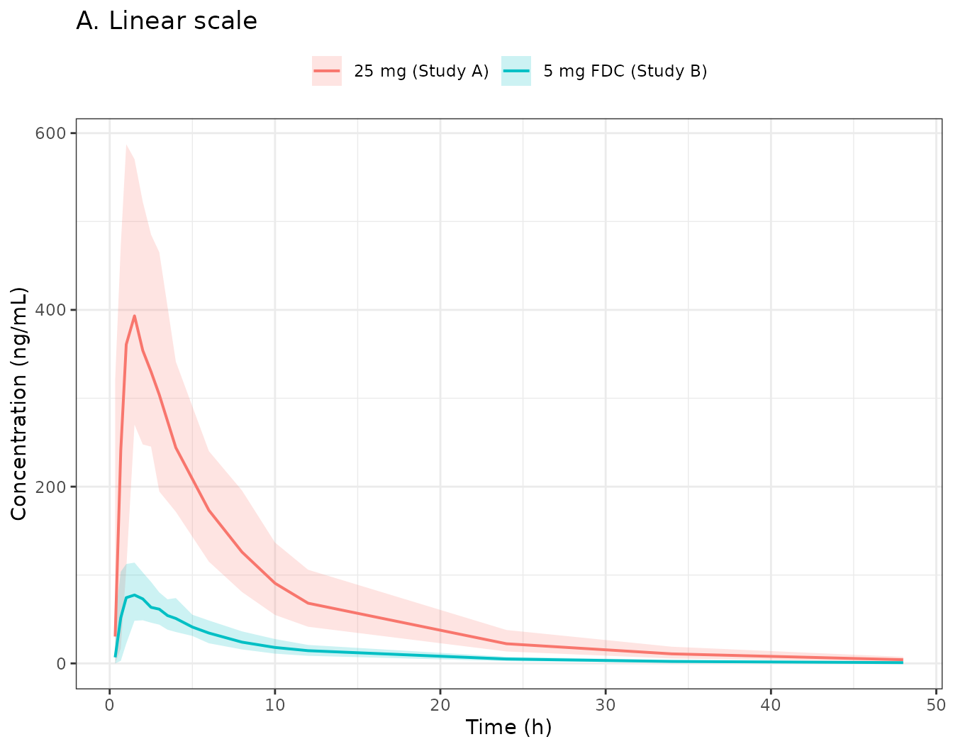
print(p_log)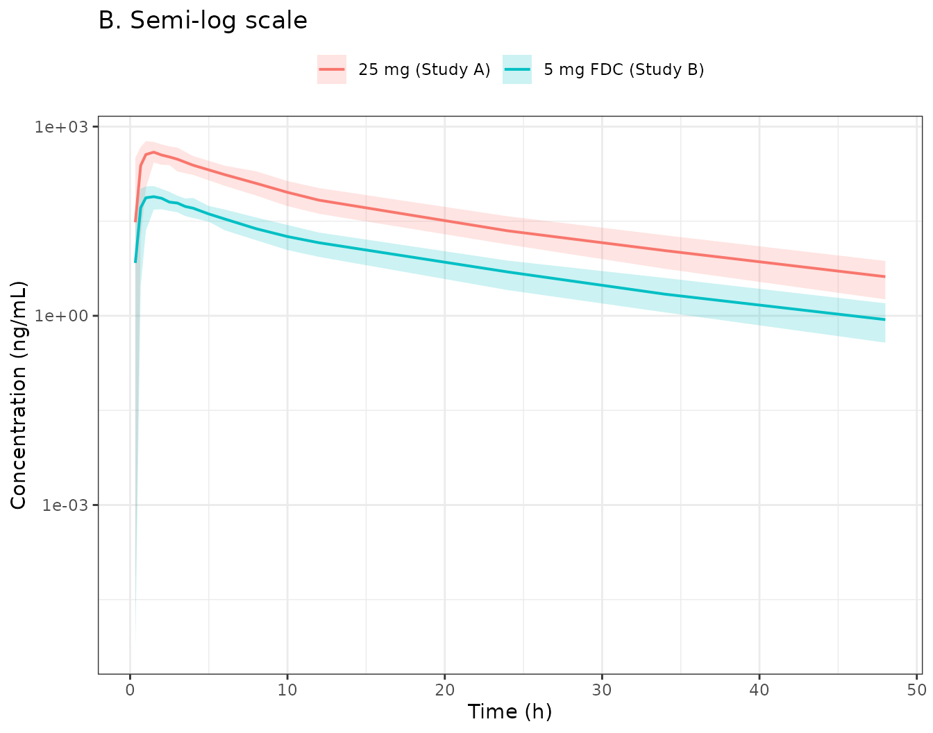
The simulated 5th-95th percentile envelope for the 25 mg arm peaks in the several-hundred ng/mL range and decays to roughly ten ng/mL by 48 h, matching the vertical extent and the shape of Jiang 2024 Figure 4 panels A and B. The observed data points of that figure cannot be overlaid because the participant data are not public.
# Illustrates the absorption chain of Figure 1 / Formula (1): the gamma-density
# transit input rate into the depot, at the typical Ktr and Mtt.
tt <- seq(0.001, 6, by = 0.005)
nn_pop <- ktr_pop * mtt_pop - 1
rate <- 25 * exp(log(ktr_pop) + nn_pop * log(ktr_pop * tt) -
                   ktr_pop * tt - lgamma(nn_pop + 1))

# The gamma density integrates to the full dose: a mass-balance check on the
# encoded absorption term.
stopifnot(abs(trapezoid(tt, rate) / 25 - 1) < 0.01)

ggplot(tibble::tibble(tt, rate), aes(tt, rate)) +
  geom_line(linewidth = 0.7) +
  geom_vline(xintercept = mtt_pop, linetype = "dashed") +
  annotate("text", x = mtt_pop + 0.12, y = max(rate) * 0.9, hjust = 0,
           label = sprintf("Mtt = %.2f h (%.1f min)", mtt_pop, mtt_pop * 60)) +
  labs(x = "Time after dose (h)", y = "Transit input rate (mg/h)",
       title = sprintf("Savic transit input, Ktr = %.2f 1/h, N = %.2f", ktr_pop, nn_pop),
       caption = "Absorption chain of Jiang 2024 Figure 1; N derived via Formula (1).") +
  theme_bw()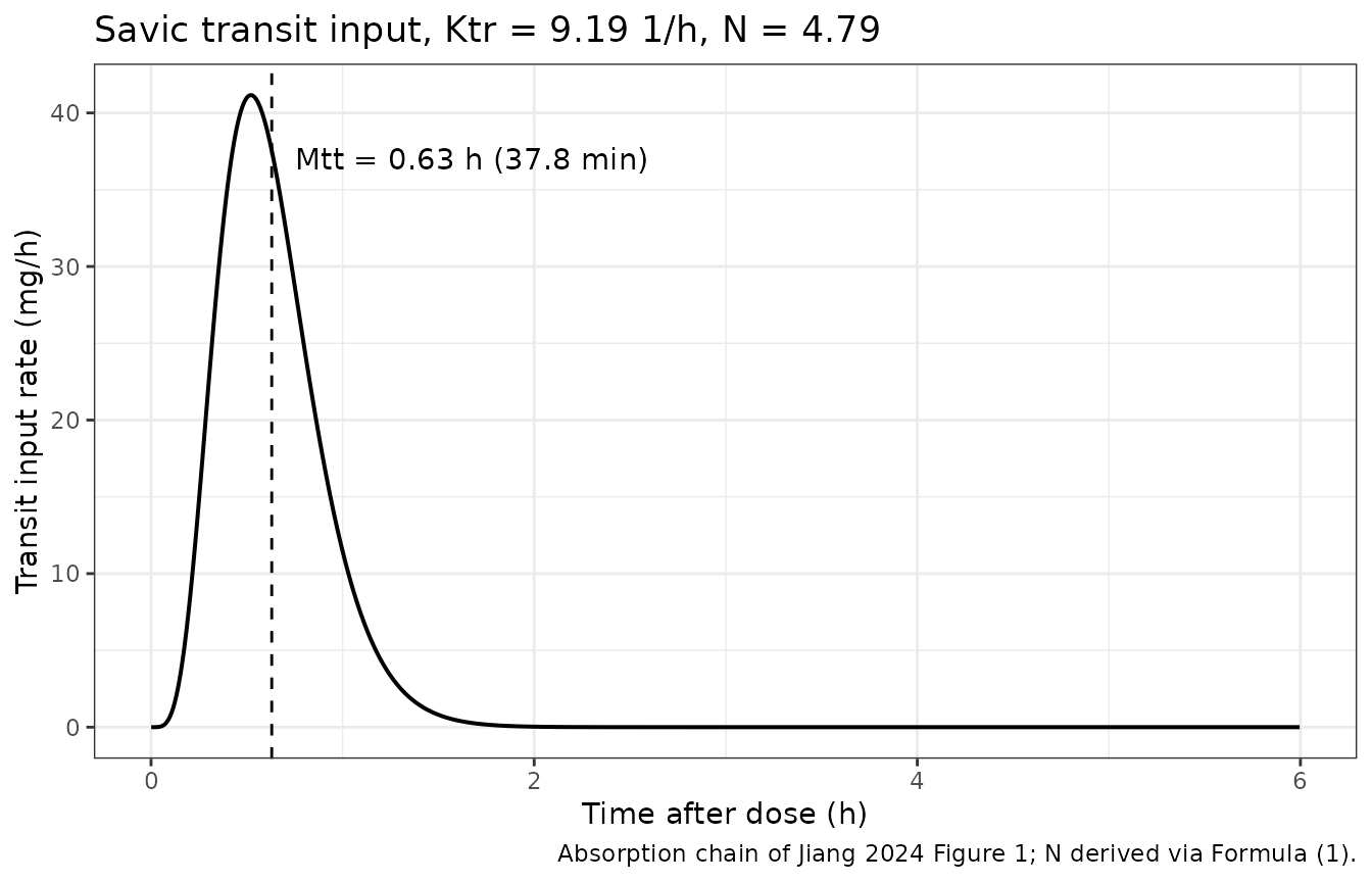
PKNCA validation
NCA is run on the individual predictions (Cc,
i.e. IPRED) converted to the ng/mL units the paper reports, over the
paper’s own sampling schedules.
sim_nca <- sim_ok |>
  filter(!is.na(Cc)) |>
  transmute(id, time, treatment, Cc = Cc * 1000)  # mg/L -> ng/mL

# Guarantee a time-zero record per subject; pre-dose Cc = 0 is correct for an
# extravascular dose. Filtering on `time > 0` or `Cc > 0` here would drop it and
# trigger PKNCA's "AUC range starting before the first measurement" warning.
sim_nca <- bind_rows(
  sim_nca,
  sim_nca |> distinct(id, treatment) |> mutate(time = 0, Cc = 0)
) |>
  distinct(id, treatment, time, .keep_all = TRUE) |>
  arrange(id, treatment, time)

dose_df <- events |>
  filter(evid == 1, !id %in% bad_ids) |>
  select(id, time, amt, treatment)

conc_obj <- PKNCA::PKNCAconc(sim_nca, Cc ~ time | treatment + id)
dose_obj <- PKNCA::PKNCAdose(dose_df, amt ~ time | treatment + id)

intervals <- data.frame(
  start = 0, end = Inf,
  cmax = TRUE, tmax = TRUE, auclast = TRUE, aucinf.obs = TRUE, half.life = TRUE
)

nca_res <- PKNCA::pk.nca(PKNCA::PKNCAdata(conc_obj, dose_obj, intervals = intervals))

nca_summary <- as.data.frame(nca_res) |>
  filter(start == 0, end == Inf) |>
  group_by(treatment, PPTESTCD) |>
  summarise(
    median = median(PPORRES, na.rm = TRUE),
    p05    = quantile(PPORRES, 0.05, na.rm = TRUE),
    p95    = quantile(PPORRES, 0.95, na.rm = TRUE),
    .groups = "drop"
  )

nca_summary |>
  mutate(across(c(median, p05, p95), \(x) signif(x, 4))) |>
  rename("Treatment" = treatment, "NCA parameter" = PPTESTCD,
         "Median" = median, "5th pctile" = p05, "95th pctile" = p95) |>
knitr::kable(caption = "Cohort NCA (IPRED scale, ng/mL) across the virtual cohort.")| Treatment | NCA parameter | Median | 5th pctile | 95th pctile |
|---|---|---|---|---|
| 25 mg (Study A) | adj.r.squared | 9.997e-01 | 9.990e-01 | 1.0000 |
| 25 mg (Study A) | aucinf.obs | 3.089e+03 | 2.357e+03 | 4001.0000 |
| 25 mg (Study A) | auclast | 3.025e+03 | 2.322e+03 | 3889.0000 |
| 25 mg (Study A) | clast.obs | 4.296e+00 | 1.864e+00 | 7.9340 |
| 25 mg (Study A) | clast.pred | 4.269e+00 | 1.863e+00 | 7.9240 |
| 25 mg (Study A) | cmax | 4.111e+02 | 3.030e+02 | 544.7000 |
| 25 mg (Study A) | half.life | 9.817e+00 | 7.850e+00 | 12.2100 |
| 25 mg (Study A) | lambda.z | 7.061e-02 | 5.679e-02 | 0.0883 |
| 25 mg (Study A) | lambda.z.n.points | 3.000e+00 | 3.000e+00 | 3.0000 |
| 25 mg (Study A) | lambda.z.time.first | 2.400e+01 | 2.400e+01 | 24.0000 |
| 25 mg (Study A) | lambda.z.time.last | 4.800e+01 | 4.800e+01 | 48.0000 |
| 25 mg (Study A) | r.squared | 9.999e-01 | 9.995e-01 | 1.0000 |
| 25 mg (Study A) | span.ratio | 2.445e+00 | 1.966e+00 | 3.0570 |
| 25 mg (Study A) | tlast | 4.800e+01 | 4.800e+01 | 48.0000 |
| 25 mg (Study A) | tmax | 1.500e+00 | 6.700e-01 | 2.0000 |
| 5 mg FDC (Study B) | adj.r.squared | 9.997e-01 | 9.990e-01 | 1.0000 |
| 5 mg FDC (Study B) | aucinf.obs | 6.176e+02 | 4.713e+02 | 800.2000 |
| 5 mg FDC (Study B) | auclast | 6.048e+02 | 4.643e+02 | 777.5000 |
| 5 mg FDC (Study B) | clast.obs | 8.593e-01 | 3.728e-01 | 1.5870 |
| 5 mg FDC (Study B) | clast.pred | 8.538e-01 | 3.725e-01 | 1.5850 |
| 5 mg FDC (Study B) | cmax | 8.222e+01 | 6.059e+01 | 108.9000 |
| 5 mg FDC (Study B) | half.life | 9.817e+00 | 7.850e+00 | 12.2100 |
| 5 mg FDC (Study B) | lambda.z | 7.061e-02 | 5.679e-02 | 0.0883 |
| 5 mg FDC (Study B) | lambda.z.n.points | 3.000e+00 | 3.000e+00 | 3.0000 |
| 5 mg FDC (Study B) | lambda.z.time.first | 2.400e+01 | 2.400e+01 | 24.0000 |
| 5 mg FDC (Study B) | lambda.z.time.last | 4.800e+01 | 4.800e+01 | 48.0000 |
| 5 mg FDC (Study B) | r.squared | 9.999e-01 | 9.995e-01 | 1.0000 |
| 5 mg FDC (Study B) | span.ratio | 2.445e+00 | 1.966e+00 | 3.0570 |
| 5 mg FDC (Study B) | tlast | 4.800e+01 | 4.800e+01 | 48.0000 |
| 5 mg FDC (Study B) | tmax | 1.500e+00 | 6.700e-01 | 2.0000 |
Comparison against reference values
Jiang 2024 reports no NCA table: no Cmax, Tmax, AUC, or half-life values appear anywhere in the paper for either dose strength. The reference column below is therefore built from the paper’s own Table 2 rather than transcribed from a published NCA table, and each entry has one of two provenances:
-
aucinf.obsandhalf.lifeare exact algebraic consequences of Table 2:AUCinf = Dose/CLand the terminal half-lifelog(2)/lambda2computed from CL, V1, V2, and Q. -
cmaxandtmaxare the typical-value predictions run through the same PKNCA pipeline on the same sampling schedule, so the comparison is NCA-to-NCA and free of sampling-grid artefacts. They test whether the cohort median tracks the typical subject, not whether the model matches an independent measurement.
typical_nca <- function(dose_mg, treatment, times) {
  ev <- bind_rows(
    tibble::tibble(WT = 70, OCC = 1L, id = 1L, time = 0, evid = 1L,
                   amt = dose_mg, cmt = "depot"),
    tibble::tibble(WT = 70, OCC = 1L, id = 1L, time = times, evid = 0L,
                   amt = NA_real_, cmt = "central")
  ) |>
    bind_cols(as.data.frame(eta_zero)[rep(1, length(times) + 1), ]) |>
    arrange(time, desc(evid))

  s <- rxode2::rxSolve(mod, ev, omega = NA, atol = 1e-12, rtol = 1e-12) |>
    as.data.frame() |>
    transmute(id = 1L, time, treatment, Cc = Cc * 1000)

  r <- PKNCA::pk.nca(PKNCA::PKNCAdata(
    PKNCA::PKNCAconc(s, Cc ~ time | treatment + id),
    PKNCA::PKNCAdose(
      tibble::tibble(id = 1L, time = 0, amt = dose_mg, treatment = treatment),
      amt ~ time | treatment + id
    ),
    intervals = intervals
  ))
  as.data.frame(r) |> filter(start == 0, end == Inf)
}

typ_nca <- bind_rows(
  typical_nca(25, "25 mg (Study A)",    times_studyA),
  typical_nca(5,  "5 mg FDC (Study B)", times_studyB)
)
pick <- function(trt, code) {
  typ_nca$PPORRES[typ_nca$treatment == trt & typ_nca$PPTESTCD == code][1]
}

published <- tibble::tribble(
  ~treatment,            ~cmax,                          ~tmax,
  "25 mg (Study A)",     pick("25 mg (Study A)", "cmax"),    pick("25 mg (Study A)", "tmax"),
  "5 mg FDC (Study B)",  pick("5 mg FDC (Study B)", "cmax"), pick("5 mg FDC (Study B)", "tmax")
) |>
  mutate(
    aucinf.obs = 1000 * c(25, 5) / cl_pop,   # Dose/CL from Table 2, in ng*h/mL
    half.life  = t_half_terminal             # log(2)/lambda2 from Table 2
  )

cmp <- nlmixr2lib::ncaComparisonTable(
  simulated = nca_res,
  reference = published,
  by        = "treatment",
  units     = c(cmax = "ng/mL", aucinf.obs = "ng*h/mL",
                tmax = "h", half.life = "h"),
  tolerance_pct = 20
)

knitr::kable(
  cmp,
  caption = paste("Cohort-median NCA vs reference values derived from Jiang 2024",
                  "Table 2. * differs from reference by >20%."),
  align = c("l", "l", "r", "r", "r")
)| NCA parameter | treatment | Reference | Simulated | % diff |
|---|---|---|---|---|
| Cmax (ng/mL) | 25 mg (Study A) | 411 | 411 | +0.1% |
| Cmax (ng/mL) | 5 mg FDC (Study B) | 82.1 | 82.2 | +0.1% |
| Tmax (h) | 25 mg (Study A) | 1.5 | 1.5 | +0.0% |
| Tmax (h) | 5 mg FDC (Study B) | 1.5 | 1.5 | +0.0% |
| AUC0-∞ (obs) (ng*h/mL) | 25 mg (Study A) | 3050 | 3090 | +1.4% |
| AUC0-∞ (obs) (ng*h/mL) | 5 mg FDC (Study B) | 609 | 618 | +1.4% |
| t½ (h) | 25 mg (Study A) | 10.1 | 9.82 | -2.5% |
| t½ (h) | 5 mg FDC (Study B) | 10.1 | 9.82 | -2.5% |
# The AUC identity is the strongest available gate: for this linear model the
# cohort-median AUCinf must sit close to Dose/CL for both dose strengths.
auc_med <- nca_summary |> filter(PPTESTCD == "aucinf.obs")
auc_ref <- setNames(1000 * c(25, 5) / cl_pop,
                    c("25 mg (Study A)", "5 mg FDC (Study B)"))
rel_err <- abs(auc_med$median / auc_ref[auc_med$treatment] - 1)
stopifnot(all(rel_err < 0.10))

# Dose proportionality must survive in the cohort too, because the 25 mg and
# 5 mg arms share eta and weight values (common random numbers).
auc_ratio <- auc_med$median[auc_med$treatment == "25 mg (Study A)"] /
  auc_med$median[auc_med$treatment == "5 mg FDC (Study B)"]
stopifnot(abs(auc_ratio - 5) < 0.05)

cat(sprintf("cohort-median AUCinf vs Dose/CL: max relative error %.2f%%\n",
            100 * max(rel_err)))
#> cohort-median AUCinf vs Dose/CL: max relative error 1.44%
cat(sprintf("cohort-median AUCinf ratio 25 mg : 5 mg = %.4f (expected 5)\n", auc_ratio))
#> cohort-median AUCinf ratio 25 mg : 5 mg = 5.0014 (expected 5)
Assumptions and deviations
- Reference weight for the covariate model is assumed. Jiang 2024 reports the coefficients on log-transformed body weight (0.64 on CL, 0.57 on the peripheral volume) but never states the centering weight, and Monolix does not fix one by convention. This model uses 70 kg, the nlmixr2lib default for an unreported centering value, which also happens to coincide with Table 1’s pooled mean weight of 69.69 kg. The pooled median of 72.1 kg is the other plausible reading; because weight enters as a power, the choice only rescales the typical values, and across the observed 55.6-83.4 kg range the two readings differ by at most 1.9% on CL and 1.7% on the peripheral volume. No parameter was tuned to compensate.
- The V1/V2 split is only weakly identified in the source. Table 2 gives V1 = 0.6 L with a bootstrap 95% CI of 0-1.889 that includes zero, against V2 = 44.6 L. The values are encoded exactly as published. Users should treat CL (RSE 1.78%) and the total Vss of 45.2 L as the well-determined quantities and the central/peripheral split as poorly constrained. Because the central compartment is small and equilibrates with the peripheral compartment within minutes (k12 = 8.2 1/h), the observable concentration is governed by V1 + V2 rather than by V1 alone, so predictions remain sensible.
-
The absorption term is written out instead of calling
transit(). Under rxode2 5.1.8,transit()combined withf(depot) <- 0silently delivers zero dose for models in nlmixr2 UI form. The explicit gamma density is algebraically identical; the “Equivalence” section above asserts agreement to better than 1e-8 mg/L against the macro. -
The very large IOV on Ktr makes both tails of the absorption
distribution numerically awkward, and this needs care when
simulating. The published gamma_Ktr of 1.17 (171% CV) is far
larger than the IOV on any other parameter, and because the chain length
is derived as N = Ktr*Mtt - 1, both tails misbehave:
- Lower tail (N < 0). The gamma input density becomes singular at t -> 0 and a fraction of occasions cannot be integrated at all; rxSolve returns NA for them rather than erroring.
-
Upper tail (large N). The input becomes a
near-impulse of width about Mtt/sqrt(N). With the default adaptive step
size the solver can step straight over it and deliver essentially no
dose, producing Cmax values around 1e-70 with no warning at all. Left
unhandled these sit in the cohort as silent zeros: on this cohort 6 of
50 occasions were affected and the median Cmax was depressed by roughly
7%. The cohort simulation therefore passes
hmax = 0.05to bound the step size, and additionally screens for undelivered doses as a standing guard. Both counts are printed in the “Cohort simulation” section and the affected occasions are excluded from the figures and NCA rather than dropped silently. This is a property of the published parameter set, not of the encoding: the typical-value profiles and every identity gate above are unaffected, since at the typical Ktr and Mtt the derived N is a well-behaved 4.79.
-
IOV etas are not mu-referenced. Multiplexing
per-occasion etas through
oc1/oc2indicators makes nlmixr2 report that these etas “defaulted to non-mu referenced”. That affects estimation efficiency if the model is re-fit, not simulation, and it matches the existing idiom inSmythe_2013_gatifloxacin.RandGoggin_2004_emfilermin.R, which produce the same message. -
Occasion 2 IOV variances are fixed equal to occasion
1. Table 2 reports one IOV standard deviation per parameter,
shared across occasions, so the occasion-2 entries use
fix()at the occasion-1 value (the NONMEM$OMEGA BLOCK(1) SAMEidiom, which nlmixr2 has no shortcut for). -
Two screened covariates with real signal could not be
encoded. Results 2.3 reports that sex on the peripheral volume
and ALP on Q both significantly improved the fit but were dropped, sex
for imprecision (RSE > 70%) and ALP as not clinically relevant.
Neither point estimate is published, so neither can be included even
optionally. Both are recorded in the model’s
covariatesDataExcludedmetadata alongside the other ten screened-but-rejected covariates. - No external validation is possible from this paper. The two source clinical studies (references 25 and 26 of Jiang 2024) hold the NCA tables for the 25 mg and 5 mg arms but are separate publications and were not available when this model was packaged. The comparison table above is consequently built from Table 2’s own algebraic consequences, and Figure 4A is used only as a qualitative concentration-scale anchor.
- Metformin is not modelled. Study B dosed empagliflozin as a fixed-dose combination with metformin 1000 mg. Jiang 2024 pooled those data on the argument that the two drugs share no metabolic pathway or transporter, and reports that estimates were similar with and without Study B. The packaged model therefore describes empagliflozin only, and the 5 mg arm here represents the empagliflozin moiety of that combination.