Iohexol in dogs (Baklouti 2021) • nlmixr2lib

Model and source

ui <- rxode2::rxode(readModelDb("Baklouti_2021_iohexol_dog"))
#> ℹ parameter labels from comments will be replaced by 'label()'

Citation: Baklouti S, Concordet D, Borromeo V, Pocar P, Scarpa P, Cagnardi P. Population pharmacokinetic model of iohexol in dogs to estimate glomerular filtration rate and optimize sampling time. Front Pharmacol. 2021;12:634404. doi:10.3389/fphar.2021.634404. All parameter values are the final estimates of Table 2; the covariate equation is the display equation of Results, ‘Population Pharmacokinetics’.
Article: https://doi.org/10.3389/fphar.2021.634404
PubMed Central: https://www.ncbi.nlm.nih.gov/pmc/articles/PMC8116701/

Iohexol is a radiographic contrast agent that is eliminated almost entirely by glomerular filtration, so its plasma clearance is a direct measure of the glomerular filtration rate (GFR). Baklouti and colleagues gave a single 64.7 mg/kg intravenous bolus of iohexol to 49 client-owned dogs, fitted a two-compartment population PK model in Monolix, and then used the model to choose the one, two or three sampling times that estimate an individual dog’s clearance (its GFR) most precisely.

All four disposition parameters are published per kg body weight, so this model is dosed in mg/kg, carries compartment amounts in mg/kg, and reports concentrations in ug/mL (equivalently mg/L) with no scaling factor. Time is in minutes. The individual clearance cl is the dog’s GFR in L/min/kg.

str(ui$units)
#> List of 3
#>  $ time         : chr "min"
#>  $ dosing       : chr "mg/kg"
#>  $ concentration: chr "ug/mL"

Population

49 client-owned dogs scheduled for various clinical procedures at the University Veterinary Teaching Hospital of the University of Milan were enrolled (Methods, “Animals”; Table 1). Ten were mongrels and 39 represented 21 pure breeds. Age ranged from 0.4 to 16 years (median 4.5) and body weight from 3.9 to 46 kg (median 27.6). Nineteen dogs were male, 6 female and 24 female neutered. By the International Renal Interest Society (IRIS) guidelines, 29 dogs had healthy kidney status (CKD-) and 20 had chronic kidney disease (CKD+). Serum creatinine was 1.47 +/- 1.99 mg/dL (range 0.67-14.4, median 1.09) and serum urea 44.95 +/- 34.81 mg/dL.

Each dog gave five plasma samples at 5, 15, 60, 90 and 180 min, 245 samples in all, assayed by HPLC (LOQ 1.80 ug/mL). The same information is available programmatically:

str(readModelDb("Baklouti_2021_iohexol_dog")()$population)
#> List of 14
#>  $ species       : chr "dog (client-owned Canis lupus familiaris; 10 mongrels and 39 dogs across 21 pure breeds)"
#>  $ n_subjects    : int 49
#>  $ n_studies     : int 1
#>  $ n_observations: int 245
#>  $ age_range     : chr "0.4-16 years"
#>  $ age_median    : chr "4.5 years"
#>  $ weight_range  : chr "3.9-46 kg"
#>  $ weight_median : chr "27.6 kg"
#>  $ sex_female_pct: num 61.2
#>  $ disease_state : chr "29 dogs with healthy kidney status (CKD-) and 20 with chronic kidney disease (CKD+) by IRIS criteria, all sched"| __truncated__
#>  $ dose_range    : chr "64.7 mg/kg (nominal) iohexol as a single 60-s intravenous bolus"
#>  $ regions       : chr "Italy (University Veterinary Teaching Hospital, University of Milan)"
#>  $ renal_function: chr "Serum creatinine 1.47 +/- 1.99 mg/dL, range 0.67-14.4 mg/dL, median 1.09 mg/dL; serum urea 44.95 +/- 34.81 mg/dL (Table 1)"
#>  $ notes         : chr "Demographics from Table 1 and Results, 'Animals and Iohexol Concentrations'. Five plasma samples per dog at 5, "| __truncated__

Nine covariates were screened: weight, age, creatinine, urea and urine specific gravity as continuous covariates, and kidney status, sex and breed as categorical ones. The final model keeps two, both on clearance: centred serum creatinine (CREAT, mg/dL) and chronic kidney disease (DIS_RENAL, 1 = CKD+). The screened-out covariates are documented in the model file’s covariatesDataExcluded metadata:

names(readModelDb("Baklouti_2021_iohexol_dog")()$covariateData)
#> [1] "CREAT"     "DIS_RENAL"
names(readModelDb("Baklouti_2021_iohexol_dog")()$covariatesDataExcluded)
#> [1] "WT"             "AGE"            "UREA"           "USG"           
#> [5] "SEXF"           "NEUTERED"       "BREED_PUREBRED"

Source trace

Equation / parameter	Value	Source location
Two-compartment disposition, IV bolus into `central`	n/a	Results, “Population Pharmacokinetics” (“A two-compartment model best fitted the data”) and Discussion (“a two-compartment model with a linear elimination”)
Individual parameters `phi_i = h(A_i, theta) exp(eta_i)`	n/a	Methods, “Population Pharmacokinetics”, model display equation
`lcl` (theta_Cl)	0.00212 L/min/kg	Table 2 (SE 0.00010, RSE 4.68%)
`lvc` (theta_V1)	0.163 L/kg	Table 2 (SE 0.00661, RSE 4.07%)
`lvp` (theta_V2)	0.058 L/kg	Table 2 (SE 0.00387, RSE 6.64%)
`lq` (theta_Q)	0.0034 L/min/kg	Table 2 (SE 0.00042, RSE 12.21%)
Covariate model `ln(Cl) = ln(theta_Cl) + theta_1 1[CKD+] + theta_2 ccreatinine + eta_Cl`	n/a	Results, “Population Pharmacokinetics”, display equation
`e_dis_renal_cl` (theta_1)	-0.379	Table 2, row “theta 1 (diseased dogs)” (SE 0.07002, RSE 18.49%)
`e_creat_cl` (theta_2)	-0.421 dL/mg	Table 2, row “theta 2 (creatinine)” (SE 0.05356, RSE 12.72%)
Creatinine centring value	1.47 mg/dL	Not printed (“centered around an average value”); Table 1 cohort mean. Confirmed by the Table 3 reproduction below
`etalcl` variance	0.208^2	Table 2, row “eta Cl” = 0.208, a Monolix standard deviation
`etalvc` variance	0.248^2	Table 2, row “eta V1” = 0.248 (SD)
`etalvp` variance	0.199^2	Table 2, row “eta V2” = 0.199 (SD)
No IIV on Q, no correlations	n/a	Discussion (“except intercompartmental clearance that was fixed”); Results (“correlations … were low (< 30%) and were therefore not included”)
`propSd`	0.0617	Table 2, row “Residual error”; Results (“proportional error … The value of the residual error was 6.17%”)
Dose	64.7 mg/kg IV bolus over 60 s	Methods, “Sample Collection and Analysis”; Supplementary File S1
EBE objective and MSE_K	n/a	Methods, “Optimal Sampling Time”, eq. 1, eq. 2 and the MSE_K display equation

Monolix reports each omega as the standard deviation of its random effect, and the Discussion reads Table 2 back that way (“the interindividual variability was around 20% on all the parameters” and RSEs “for the standard deviation of the random effects”). The variances in ini() are therefore the squared Table 2 values. The reproduction of Table 3 below confirms this reading: that table depends directly on the size of the IIV relative to the residual error.

omega <- ui$omega
sd_published <- c(etalcl = 0.208, etalvc = 0.248, etalvp = 0.199)
knitr::kable(
  data.frame(
    `Random effect` = names(sd_published),
    `Table 2 (SD)` = unname(sd_published),
    `sqrt(model variance)` = unname(sqrt(diag(omega))[names(sd_published)]),
    check.names = FALSE
  ),
  digits = 4,
  caption = "Table 2 IIV standard deviations versus the packaged variances."
)

Table 2 IIV standard deviations versus the packaged variances.
Random effect	Table 2 (SD)	sqrt(model variance)
etalcl	0.208	0.208
etalvc	0.248	0.248
etalvp	0.199	0.199

# Deterministic arithmetic on transcribed constants: a tight bound is correct.
stopifnot(
  identical(sort(rownames(omega)), sort(names(sd_published))),
  max(abs(sqrt(diag(omega))[names(sd_published)] - sd_published)) < 1e-9
)

The three example dogs

The paper illustrates its sampling-time analysis with three example dogs that span renal function (Methods, “Optimal Sampling Time”). Their typical-value clearances follow directly from the Table 2 constants and the covariate equation.

theta <- setNames(ui$theta, names(ui$theta))
creat_ref <- 1.47

examples <- tibble::tibble(
  treatment = c(
    "Example 1: CKD-, creatinine 0.98",
    "Example 2: CKD+, creatinine 1.7",
    "Example 3: CKD+, creatinine 2.25"
  ),
  DIS_RENAL = c(0, 1, 1),
  CREAT = c(0.98, 1.7, 2.25)
) |>
  dplyr::mutate(
    id = dplyr::row_number(),
    cl_typical = exp(
      theta[["lcl"]] + theta[["e_dis_renal_cl"]] * DIS_RENAL +
        theta[["e_creat_cl"]] * (CREAT - creat_ref)
    )
  )

knitr::kable(
  examples |>
    dplyr::select(treatment, DIS_RENAL, CREAT, cl_typical) |>
    dplyr::mutate(`GFR (mL/min/kg)` = 1000 * cl_typical) |>
    dplyr::rename(
      Dog = treatment,
      `CKD (DIS_RENAL)` = DIS_RENAL,
      `Creatinine (mg/dL)` = CREAT,
      `Typical CL (L/min/kg)` = cl_typical
    ),
  digits = 5,
  caption = "Typical clearance (GFR) of the three example dogs of Baklouti 2021."
)

Typical clearance (GFR) of the three example dogs of Baklouti 2021.
Dog	CKD (DIS_RENAL)	Creatinine (mg/dL)	Typical CL (L/min/kg)	GFR (mL/min/kg)
Example 1: CKD-, creatinine 0.98	0	0.98	0.00261	2.60571
Example 2: CKD+, creatinine 1.7	1	1.70	0.00132	1.31730
Example 3: CKD+, creatinine 2.25	1	2.25	0.00105	1.04502

The typical profiles are simulated with the random effects zeroed. The same profiles are also computed from the closed-form biexponential solution of an IV bolus into a two-compartment model; the closed form is reused below for the sampling-time analysis, so it is checked against the ODE solve first.

dose_mgkg <- 64.7
obs_times <- c(0, 1, 2, 5, 10, 15, seq(20, 180, by = 5))

events_typ <- dplyr::bind_rows(
  examples |> dplyr::mutate(time = 0, amt = dose_mgkg, evid = 1L, cmt = "central"),
  tidyr::crossing(examples, tibble::tibble(time = obs_times)) |>
    dplyr::mutate(amt = NA_real_, evid = 0L, cmt = "central")
) |>
  dplyr::select(id, time, amt, evid, cmt, DIS_RENAL, CREAT) |>
  dplyr::arrange(id, time, dplyr::desc(evid))

sim_typ <- rxode2::rxSolve(
  rxode2::zeroRe(ui),
  events = events_typ,
  keep = c("DIS_RENAL", "CREAT"),
  returnType = "data.frame"
) |>
  dplyr::left_join(examples |> dplyr::select(id, treatment), by = "id")
#> ℹ omega/sigma items treated as zero: 'etalcl', 'etalvc', 'etalvp'
#> Warning: multi-subject simulation without without 'omega'

# Closed-form concentration for a 2-compartment IV bolus.
conc_2cmt <- function(t, dose, cl, vc, vp, q) {
  k10 <- cl / vc
  k12 <- q / vc
  k21 <- q / vp
  s <- k10 + k12 + k21
  p <- k10 * k21
  alpha <- (s + sqrt(s^2 - 4 * p)) / 2
  beta <- (s - sqrt(s^2 - 4 * p)) / 2
  dose / vc * ((alpha - k21) / (alpha - beta) * exp(-alpha * t) +
    (k21 - beta) / (alpha - beta) * exp(-beta * t))
}

closed <- sim_typ |>
  dplyr::filter(time > 0) |>
  dplyr::left_join(examples |> dplyr::select(id, cl_typical), by = "id") |>
  dplyr::mutate(
    Cc_closed = conc_2cmt(
      time, dose_mgkg, cl_typical,
      exp(theta[["lvc"]]), exp(theta[["lvp"]]), exp(theta[["lq"]])
    )
  )
# Same parameters on both sides, so the difference is pure solver error.
stopifnot(max(abs(closed$Cc / closed$Cc_closed - 1)) < 1e-4)

ggplot(sim_typ |> dplyr::filter(time > 0), aes(time, Cc, colour = treatment)) +
  geom_line(linewidth = 0.8) +
  scale_y_log10() +
  labs(
    x = "Time after dose (min)", y = "Iohexol (ug/mL)", colour = NULL,
    title = "Typical-value iohexol profiles for the three example dogs",
    caption = "64.7 mg/kg IV bolus; random effects set to zero."
  ) +
  theme_bw() +
  theme(legend.position = "bottom", legend.direction = "vertical")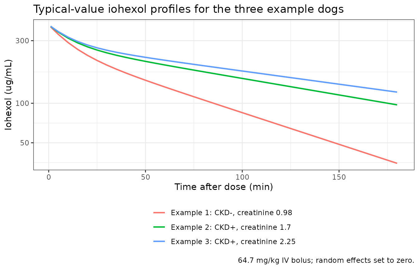

The Discussion states that “all dogs CKD+ with the high creatinine value had an iohexol concentration greater than 100 ug/ml at 180 min”. The typical example 3 dog agrees:

c180 <- sim_typ |>
  dplyr::filter(time == 180) |>
  dplyr::select(treatment, Cc)
knitr::kable(
  c180 |> dplyr::rename(Dog = treatment, `Cc at 180 min (ug/mL)` = Cc),
  digits = 1
)

Dog	Cc at 180 min (ug/mL)
Example 1: CKD-, creatinine 0.98	34.9
Example 2: CKD+, creatinine 1.7	97.3
Example 3: CKD+, creatinine 2.25	121.6

stopifnot(c180$Cc[3] > 100)

Virtual cohort and visual predictive check

Original observed data are not publicly available. Figure 3 of the paper is a visual predictive check of the observed 10th, 50th and 90th percentiles at the five sampling times. Its percentiles were digitised by the maintainers from the published figure and are compared here with a virtual cohort of 200 dogs.

The cohort needs creatinine values and kidney status. The paper gives only the pooled creatinine summary (mean 1.47, SD 1.99, median 1.09, range 0.67-14.4 mg/dL) and 20 of 49 dogs with CKD, so the maintainers assumed the split below: 82 of 200 dogs (41%) are CKD+; healthy dogs draw creatinine from a log-normal with median 0.95 mg/dL (CV about 20%) truncated to 0.67-1.39 mg/dL (IRIS stage 1 is below 1.4 mg/dL), and CKD+ dogs from a log-normal with median 1.6 mg/dL (CV about 36%) truncated to 1.0-14.4 mg/dL. This distribution is an assumption, and it mostly affects the late time points where clearance dominates.

# Covariates are drawn with base R's generator, which is identical on every
# machine. The random effects are drawn by rxode2; rxSetSeed() fixes that
# stream per solver thread but not across thread counts or rxode2 builds, so
# the assertions below tolerate any cohort the model can produce.
set.seed(20210429)
rxode2::rxSetSeed(20210429)

n_dogs <- 200L
n_ckd <- 82L
creat_healthy <- pmin(pmax(exp(rnorm(n_dogs - n_ckd, log(0.95), 0.2)), 0.67), 1.39)
creat_ckd <- pmin(pmax(exp(rnorm(n_ckd, log(1.6), 0.35)), 1.0), 14.4)

cohort <- tibble::tibble(
  id = seq_len(n_dogs),
  DIS_RENAL = c(rep(0, n_dogs - n_ckd), rep(1, n_ckd)),
  CREAT = c(creat_healthy, creat_ckd),
  treatment = ifelse(DIS_RENAL == 1, "CKD+", "CKD-")
)

vpc_times <- c(5, 15, 60, 90, 180)
events_vpc <- dplyr::bind_rows(
  cohort |> dplyr::mutate(time = 0, amt = dose_mgkg, evid = 1L, cmt = "central"),
  tidyr::crossing(cohort, tibble::tibble(time = vpc_times)) |>
    dplyr::mutate(amt = NA_real_, evid = 0L, cmt = "central")
) |>
  dplyr::select(id, time, amt, evid, cmt, DIS_RENAL, CREAT) |>
  dplyr::arrange(id, time, dplyr::desc(evid))

sim_vpc <- rxode2::rxSolve(
  ui,
  events = events_vpc,
  keep = c("DIS_RENAL", "CREAT"),
  returnType = "data.frame"
)

vpc_sim <- sim_vpc |>
  dplyr::filter(time %in% vpc_times) |>
  dplyr::group_by(time) |>
  dplyr::summarise(
    p10 = quantile(sim, 0.1),
    p50 = median(sim),
    p90 = quantile(sim, 0.9),
    .groups = "drop"
  )

# Figure 3 of Baklouti 2021, empirical percentiles read off the published
# figure by the maintainers (ug/mL).
vpc_fig3 <- tibble::tibble(
  time = vpc_times,
  p10 = c(266, 202, 111, 76, 25),
  p50 = c(335, 256, 141, 100, 44),
  p90 = c(458, 325, 219, 183, 112)
)

vpc_long <- dplyr::bind_rows(
  vpc_sim |> dplyr::mutate(source = "Simulated (this model)"),
  vpc_fig3 |> dplyr::mutate(source = "Observed (Figure 3)")
) |>
  tidyr::pivot_longer(c(p10, p50, p90), names_to = "percentile", values_to = "conc")

ggplot(vpc_long, aes(time, conc, colour = source, linetype = percentile)) +
  geom_line() +
  geom_point() +
  labs(
    x = "Time after dose (min)", y = "Iohexol (ug/mL)", colour = NULL,
    linetype = "Percentile",
    title = "Replicates Figure 3 of Baklouti 2021 (visual predictive check)",
    caption = "200 virtual dogs; observed percentiles digitised from Figure 3."
  ) +
  theme_bw()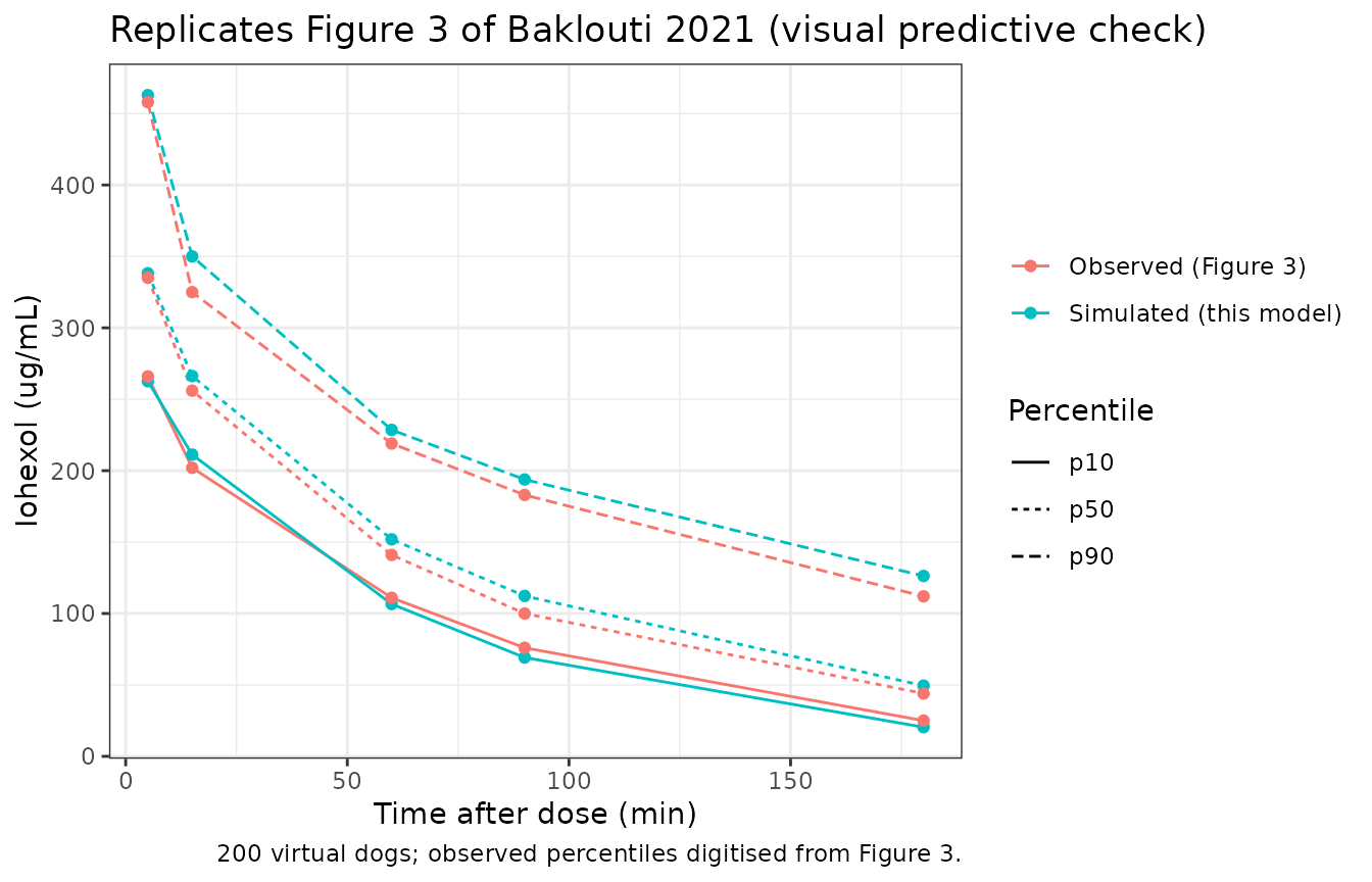


vpc_cmp <- vpc_sim |>
  dplyr::left_join(vpc_fig3, by = "time", suffix = c("_sim", "_fig3")) |>
  dplyr::mutate(pct_diff_median = 100 * (p50_sim / p50_fig3 - 1))

knitr::kable(
  vpc_cmp |>
    dplyr::select(time, p50_fig3, p50_sim, pct_diff_median, p10_fig3, p10_sim, p90_fig3, p90_sim) |>
    dplyr::rename(
      `Time (min)` = time,
      `Median, Figure 3` = p50_fig3,
      `Median, simulated` = p50_sim,
      `Median % diff` = pct_diff_median,
      `P10, Figure 3` = p10_fig3,
      `P10, simulated` = p10_sim,
      `P90, Figure 3` = p90_fig3,
      `P90, simulated` = p90_sim
    ),
  digits = 1,
  caption = "Simulated versus observed (Figure 3) percentiles, ug/mL."
)

Simulated versus observed (Figure 3) percentiles, ug/mL.
Time (min)	Median, Figure 3	Median, simulated	Median % diff	P10, Figure 3	P10, simulated	P90, Figure 3	P90, simulated
5	335	338.2	0.9	266	262.6	458	462.9
15	256	266.2	4.0	202	211.2	325	350.0
60	141	151.9	7.8	111	106.6	219	228.6
90	100	112.3	12.3	76	69.2	183	193.8
180	44	49.5	12.5	25	20.4	112	126.3


stopifnot(
  # The early times are governed by V1 and the dose, not by the assumed
  # creatinine distribution: a mis-transcribed volume or dose moves them by
  # tens of percent.
  all(abs(vpc_cmp$pct_diff_median[vpc_cmp$time <= 15]) < 15),
  # Centre of the whole comparison, robust to the assumed cohort.
  median(abs(vpc_cmp$pct_diff_median)) < 15
)

The medians agree within a few percent through 60 min. At 90 and 180 min the simulated medians sit about 10-25% above the observed ones (the exact figure depends on the random-effect draw). Those time points are driven by clearance, so they depend on the creatinine distribution of the 49 real dogs, which the paper does not publish, and the assumed cohort above may carry somewhat more low-clearance dogs than the real one did. The model’s clearance is validated independently of any assumed cohort by the reproduction of Table 3 below.

PKNCA validation

Iohexol clearance measured by NCA as dose / AUC0-inf is the GFR reference method the paper compares against (Pocar 2019; Figure 4). For each typical example dog, the NCA clearance of a densely sampled simulated profile should equal the model clearance of the table above. That comparison checks the dose, the units and the covariate equation together.

nca_times <- c(0, 1, 2, 5, 10, 15, 20, 30, 45, seq(60, 1440, by = 30))

events_nca <- dplyr::bind_rows(
  examples |> dplyr::mutate(time = 0, amt = dose_mgkg, evid = 1L, cmt = "central"),
  tidyr::crossing(examples, tibble::tibble(time = nca_times)) |>
    dplyr::mutate(amt = NA_real_, evid = 0L, cmt = "central")
) |>
  dplyr::select(id, time, amt, evid, cmt, DIS_RENAL, CREAT) |>
  dplyr::arrange(id, time, dplyr::desc(evid))

sim_nca <- rxode2::rxSolve(
  rxode2::zeroRe(ui),
  events = events_nca,
  keep = c("DIS_RENAL", "CREAT"),
  returnType = "data.frame"
) |>
  dplyr::left_join(examples |> dplyr::select(id, treatment), by = "id")
#> ℹ omega/sigma items treated as zero: 'etalcl', 'etalvc', 'etalvp'
#> Warning: multi-subject simulation without without 'omega'

conc_df <- sim_nca |>
  dplyr::filter(!is.na(Cc)) |>
  dplyr::select(id, treatment, time, Cc)
# The bolus gives a non-zero concentration at time 0; PKNCA back-extrapolates
# C0 for an IV bolus, so the time-0 row is kept as simulated.
dose_df <- examples |>
  dplyr::transmute(id, treatment, time = 0, amt = dose_mgkg)

conc_obj <- PKNCA::PKNCAconc(conc_df, Cc ~ time | treatment + id)
dose_obj <- PKNCA::PKNCAdose(dose_df, amt ~ time | treatment + id, route = "intravascular")
intervals <- data.frame(
  start = 0, end = Inf,
  cmax = TRUE, aucinf.obs = TRUE, half.life = TRUE, cl.obs = TRUE
)
nca_res <- PKNCA::pk.nca(PKNCA::PKNCAdata(conc_obj, dose_obj, intervals = intervals))

reference <- examples |>
  dplyr::transmute(
    treatment,
    cl.obs = cl_typical,
    aucinf.obs = dose_mgkg / cl_typical
  )

nca_units <- c(cl.obs = "L/min/kg", aucinf.obs = "ug*min/mL")
cmp <- nlmixr2lib::ncaComparisonTable(
  simulated = nca_res,
  reference = reference,
  by = "treatment",
  params = c("aucinf.obs", "cl.obs"),
  units = nca_units,
  tolerance_pct = 20
)
knitr::kable(
  cmp,
  caption = "PKNCA on the typical example dogs versus the Table 2 clearance (reference = dose / CL).",
  align = c("l", "l", "r", "r", "r")
)

PKNCA on the typical example dogs versus the Table 2 clearance (reference = dose / CL).
NCA parameter	treatment	Reference	Simulated	% diff
AUC0-∞ (obs) (ug*min/mL)	Example 1: CKD-, creatinine 0.98	24800	24900	+0.1%
AUC0-∞ (obs) (ug*min/mL)	Example 2: CKD+, creatinine 1.7	49100	49100	+0.1%
AUC0-∞ (obs) (ug*min/mL)	Example 3: CKD+, creatinine 2.25	61900	61900	+0.1%
CL/F (L/min/kg)	Example 1: CKD-, creatinine 0.98	0.00261	0.0026	-0.1%
CL/F (L/min/kg)	Example 2: CKD+, creatinine 1.7	0.00132	0.00132	-0.1%
CL/F (L/min/kg)	Example 3: CKD+, creatinine 2.25	0.00105	0.00104	-0.1%


diff_col <- grep("diff", names(cmp), value = TRUE)
pct <- suppressWarnings(as.numeric(gsub("[%*]", "", cmp[[diff_col]])))
# Deterministic typical-value profiles sampled to 24 h: only the trapezoidal
# and extrapolation error of NCA separates the two sides.
stopifnot(length(pct) == 6L, !anyNA(pct), max(abs(pct)) < 2)

Optimal sampling times: reproducing Tables 3-5

For each example dog, the paper simulated 5,000 profiles, computed each simulated dog’s empirical Bayes estimate (EBE) of its random effects from one, two or three samples taken between 30 and 180 min, and scored each sampling design K by

$MSE_K = \frac{1}{5000}\sqrt{\sum_{i=1}^{5000}\left(\widehat{\eta}^{*}_{i,K} - \eta^{*}_i\right)^2},$

the EBE error in the clearance random effect (Methods, “Optimal Sampling Time”). Note that this “MSE” is a root-sum-of-squares divided by the number of simulations, i.e. the root-mean-square error divided by sqrt(5000); the value is reported in units of 10^-3. The EBE is the mode of the conditional distribution, which the paper writes as minimising (eq. 2)

$\sum_{t \in K} \frac{(Y_t - f_t)^2}{g_t^2} + \ln g_t^2 + \eta' \Omega^{-1} \eta, \qquad g_t = b\, f_t .$

The reproduction below uses 200 simulated dogs per example dog, draws the random effects and residuals with base R’s generator from the packaged ini() values, reuses the same draws for every design of a table (common random numbers), and scales the root-mean-square error to the paper’s 1 / sqrt(5000) form so the numbers are directly comparable. This analysis exercises the whole stochastic model – the covariate equation, the three IIV standard deviations and the 6.17% residual error – because the EBE precision is set by the ratio of the IIV to the residual error.

omega_diag <- diag(ui$omega)[c("etalcl", "etalvc", "etalvp")]
prop_sd <- theta[["propSd"]]
sampling_grid <- c(30, 60, 90, 120, 150, 180)

ind_par <- function(eta, dis_renal, creat) {
  list(
    cl = exp(theta[["lcl"]] + theta[["e_dis_renal_cl"]] * dis_renal +
      theta[["e_creat_cl"]] * (creat - creat_ref) + eta[1]),
    vc = exp(theta[["lvc"]] + eta[2]),
    vp = exp(theta[["lvp"]] + eta[3]),
    q = exp(theta[["lq"]])
  )
}

# Eq. 2 of Baklouti 2021 (the constant factor 1/2 does not move the mode).
ebe_objective <- function(eta, y, t, dis_renal, creat) {
  p <- ind_par(eta, dis_renal, creat)
  f <- conc_2cmt(t, dose_mgkg, p$cl, p$vc, p$vp, p$q)
  g2 <- (prop_sd * f)^2
  sum((y - f)^2 / g2 + log(g2)) + sum(eta^2 / omega_diag)
}

# Squared EBE error in the clearance random effect for simulated dog i under
# sampling design tk.
ebe_sq_err <- function(i, tk, eta_true, eps, dis_renal, creat) {
  idx <- match(tk, sampling_grid)
  p <- ind_par(eta_true[i, ], dis_renal, creat)
  y <- conc_2cmt(tk, dose_mgkg, p$cl, p$vc, p$vp, p$q) * (1 + prop_sd * eps[i, idx])
  fit <- stats::optim(
    c(0, 0, 0), ebe_objective,
    y = y, t = tk, dis_renal = dis_renal, creat = creat,
    method = "BFGS"
  )
  (fit$par[1] - eta_true[i, 1])^2
}

# The paper's MSE_K (x10^-3) for one design: RMSE / sqrt(5000).
mse_k <- function(tk, eta_true, eps, dis_renal, creat) {
  sq_err <- vapply(
    seq_len(nrow(eta_true)), ebe_sq_err, numeric(1),
    tk = tk, eta_true = eta_true, eps = eps,
    dis_renal = dis_renal, creat = creat
  )
  1000 * sqrt(mean(sq_err)) / sqrt(5000)
}

# One example dog: draw the true random effects and residuals once and reuse
# them for every design (common random numbers).
mse_designs <- function(j, designs, n_sim) {
  eta_true <- cbind(
    rnorm(n_sim, 0, sqrt(omega_diag[[1]])),
    rnorm(n_sim, 0, sqrt(omega_diag[[2]])),
    rnorm(n_sim, 0, sqrt(omega_diag[[3]]))
  )
  eps <- matrix(rnorm(n_sim * length(sampling_grid)), n_sim, length(sampling_grid))
  vapply(
    designs, mse_k, numeric(1),
    eta_true = eta_true, eps = eps,
    dis_renal = examples$DIS_RENAL[j], creat = examples$CREAT[j]
  )
}

run_table <- function(designs, n_sim, seed) {
  set.seed(seed)
  res <- vapply(seq_len(nrow(examples)), mse_designs, numeric(length(designs)),
    designs = designs, n_sim = n_sim
  )
  tibble::tibble(
    design = vapply(designs, paste, character(1), collapse = "_"),
    ex1 = res[, 1], ex2 = res[, 2], ex3 = res[, 3]
  )
}

n_sim_mse <- 200L
designs_1 <- as.list(sampling_grid)
designs_2 <- combn(sampling_grid, 2, simplify = FALSE)
designs_3 <- combn(sampling_grid, 3, simplify = FALSE)

The published values of Tables 3-5 (x10^-3):

published_1 <- tibble::tibble(
  design = c("30", "60", "90", "120", "150", "180"),
  ex1 = c(2.37144, 1.48213, 1.08587, 1.04398, 1.15137, 1.27023),
  ex2 = c(2.83923, 2.49541, 2.06094, 1.55052, 1.21796, 1.05704),
  ex3 = c(2.87982, 2.71283, 2.33112, 2.03204, 1.58001, 1.27007)
)
published_2 <- tibble::tibble(
  design = c(
    "30_60", "30_90", "30_120", "30_150", "30_180", "60_90", "60_120",
    "60_150", "60_180", "90_120", "90_150", "90_180", "120_150", "120_180",
    "150_180"
  ),
  ex1 = c(
    1.59044, 1.04184, 0.8313, 0.77656, 0.76386, 1.01744, 0.8628, 0.84146,
    0.83782, 0.90116, 0.89505, 0.91048, 0.99535, 1.00764, 1.17352
  ),
  ex2 = c(
    2.94597, 2.02553, 1.52744, 1.24404, 1.04572, 2.11078, 1.53112, 1.18311,
    1.00331, 1.65281, 1.23837, 1.00323, 1.22089, 0.9865, 0.97719
  ),
  ex3 = c(
    3.38164, 2.47435, 1.88487, 1.54674, 1.29145, 2.63993, 1.91978, 1.49829,
    1.21676, 2.14052, 1.6483, 1.29749, 1.67092, 1.34951, 1.24635
  )
)
published_3 <- tibble::tibble(
  design = c(
    "30_60_90", "30_60_120", "30_60_150", "30_60_180", "30_90_120",
    "30_90_150", "30_90_180", "30_120_150", "30_120_180", "30_150_180",
    "60_90_120", "60_90_150", "60_90_180", "60_120_150", "60_120_180",
    "60_150_180", "90_120_150", "90_120_180", "90_150_180", "120_150_180"
  ),
  ex1 = c(
    1.01127, 0.79361, 0.72799, 0.68501, 0.75675, 0.69878, 0.67861, 0.68581,
    0.67313, 0.67858, 0.79057, 0.75929, 0.75331, 0.76469, 0.75608, 0.77419,
    0.82071, 0.81691, 0.86003, 0.95395
  ),
  ex2 = c(
    2.00212, 1.49464, 1.20321, 0.98346, 1.43671, 1.17373, 0.97652, 1.09122,
    0.93237, 0.8623, 1.47998, 1.1665, 0.96534, 1.07649, 0.9122, 0.84264,
    1.14447, 0.94613, 0.88547, 0.884564
  ),
  ex3 = c(
    2.43594, 1.81317, 1.48077, 1.22154, 1.80194, 1.45919, 1.2322, 1.38739,
    1.18603, 1.10814, 1.86321, 1.50283, 1.23779, 1.396, 1.16991, 1.08415,
    1.55208, 1.2775, 1.18735, 1.23236
  )
)

mse_1 <- run_table(designs_1, n_sim_mse, seed = 1)
mse_2 <- run_table(designs_2, n_sim_mse, seed = 2)
mse_3 <- run_table(designs_3, n_sim_mse, seed = 3)

compare_mse <- function(sim, pub, n_samples) {
  dplyr::inner_join(
    tidyr::pivot_longer(pub, -design, names_to = "example", values_to = "published"),
    tidyr::pivot_longer(sim, -design, names_to = "example", values_to = "simulated"),
    by = c("design", "example")
  ) |>
    dplyr::mutate(
      samples = n_samples,
      pct_diff = 100 * (simulated / published - 1)
    )
}

mse_cmp <- dplyr::bind_rows(
  compare_mse(mse_1, published_1, 1L),
  compare_mse(mse_2, published_2, 2L),
  compare_mse(mse_3, published_3, 3L)
)
stopifnot(nrow(mse_cmp) == 3L * (6L + 15L + 20L))

mse_wide <- mse_cmp |>
  dplyr::mutate(cell = sprintf("%.3f / %.3f", published, simulated)) |>
  dplyr::select(samples, design, example, cell) |>
  tidyr::pivot_wider(names_from = example, values_from = cell)

knitr::kable(
  mse_wide |>
    dplyr::rename(
      `Samples` = samples,
      `Times (min)` = design,
      `Example 1 (CKD-, 0.98)` = ex1,
      `Example 2 (CKD+, 1.7)` = ex2,
      `Example 3 (CKD+, 2.25)` = ex3
    ),
  caption = "Replicates Tables 3-5 of Baklouti 2021: MSE_K (x10^-3), published / simulated."
)

Replicates Tables 3-5 of Baklouti 2021: MSE_K (x10^-3), published / simulated.
Samples	Times (min)	Example 1 (CKD-, 0.98)	Example 2 (CKD+, 1.7)	Example 3 (CKD+, 2.25)
1	30	2.371 / 2.293	2.839 / 2.997	2.880 / 3.059
1	60	1.482 / 1.492	2.495 / 2.535	2.713 / 2.893
1	90	1.086 / 1.049	2.061 / 2.037	2.331 / 2.551
1	120	1.044 / 1.012	1.551 / 1.558	2.032 / 2.241
1	150	1.151 / 1.160	1.218 / 1.167	1.580 / 1.769
1	180	1.270 / 1.273	1.057 / 1.044	1.270 / 1.283
2	30_60	1.590 / 1.555	2.946 / 2.410	3.382 / 2.429
2	30_90	1.042 / 0.996	2.026 / 1.874	2.474 / 2.035
2	30_120	0.831 / 0.820	1.527 / 1.294	1.885 / 1.581
2	30_150	0.777 / 0.630	1.244 / 1.105	1.547 / 1.298
2	30_180	0.764 / 0.634	1.046 / 0.891	1.291 / 1.055
2	60_90	1.017 / 1.012	2.111 / 2.037	2.640 / 2.313
2	60_120	0.863 / 0.860	1.531 / 1.361	1.920 / 1.742
2	60_150	0.841 / 0.693	1.183 / 1.131	1.498 / 1.406
2	60_180	0.838 / 0.747	1.003 / 0.907	1.217 / 1.086
2	90_120	0.901 / 0.902	1.653 / 1.437	2.141 / 1.800
2	90_150	0.895 / 0.803	1.238 / 1.162	1.648 / 1.459
2	90_180	0.910 / 0.806	1.003 / 0.924	1.297 / 1.104
2	120_150	0.995 / 1.073	1.221 / 1.146	1.671 / 1.495
2	120_180	1.008 / 1.081	0.987 / 0.909	1.350 / 1.126
2	150_180	1.174 / 1.130	0.977 / 0.859	1.246 / 1.123
3	30_60_90	1.011 / 0.945	2.002 / 1.687	2.436 / 2.095
3	30_60_120	0.794 / 0.716	1.495 / 1.323	1.813 / 1.638
3	30_60_150	0.728 / 0.611	1.203 / 1.043	1.481 / 1.196
3	30_60_180	0.685 / 0.576	0.983 / 0.856	1.222 / 1.020
3	30_90_120	0.757 / 0.726	1.437 / 1.267	1.802 / 1.552
3	30_90_150	0.699 / 0.623	1.174 / 1.016	1.459 / 1.184
3	30_90_180	0.679 / 0.578	0.977 / 0.835	1.232 / 0.997
3	30_120_150	0.686 / 0.629	1.091 / 0.947	1.387 / 1.127
3	30_120_180	0.673 / 0.597	0.932 / 0.774	1.186 / 0.921
3	30_150_180	0.679 / 0.591	0.862 / 0.728	1.108 / 0.830
3	60_90_120	0.791 / 0.757	1.480 / 1.299	1.863 / 1.778
3	60_90_150	0.759 / 0.669	1.167 / 1.085	1.503 / 1.320
3	60_90_180	0.753 / 0.642	0.965 / 0.859	1.238 / 1.065
3	60_120_150	0.765 / 0.665	1.076 / 0.991	1.396 / 1.294
3	60_120_180	0.756 / 0.642	0.912 / 0.801	1.170 / 1.017
3	60_150_180	0.774 / 0.657	0.843 / 0.757	1.084 / 0.935
3	90_120_150	0.821 / 0.811	1.144 / 1.061	1.552 / 1.389
3	90_120_180	0.817 / 0.774	0.946 / 0.852	1.278 / 1.044
3	90_150_180	0.860 / 0.807	0.885 / 0.787	1.187 / 0.957
3	120_150_180	0.954 / 0.894	0.885 / 0.828	1.232 / 1.057


ggplot(
  mse_cmp |> dplyr::filter(samples == 1L) |>
    dplyr::mutate(time = as.numeric(design)) |>
    tidyr::pivot_longer(c(published, simulated), names_to = "source", values_to = "mse"),
  aes(time, mse, colour = example, linetype = source)
) +
  geom_line() +
  geom_point() +
  labs(
    x = "Single sampling time (min)", y = "MSE_K (x10^-3)",
    colour = "Example dog", linetype = NULL,
    title = "Replicates Figure 5 / Table 3 of Baklouti 2021 (one sample)"
  ) +
  theme_bw()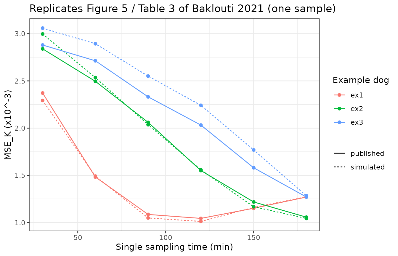


mse_summary <- mse_cmp |>
  dplyr::group_by(samples) |>
  dplyr::summarise(
    `Median % diff` = median(pct_diff),
    `Median |% diff|` = median(abs(pct_diff)),
    `90th percentile |% diff|` = quantile(abs(pct_diff), 0.9),
    .groups = "drop"
  )
knitr::kable(mse_summary, digits = 1, caption = "Agreement with Tables 3-5 by number of samples.")

Agreement with Tables 3-5 by number of samples.
samples	Median % diff	Median \|% diff\|	90th percentile \|% diff\|
1	0.7	3.2	9.7
2	-10.7	10.7	17.7
3	-12.9	12.9	18.8


best_single <- mse_1 |>
  tidyr::pivot_longer(-design, names_to = "example", values_to = "mse") |>
  dplyr::group_by(example) |>
  dplyr::slice_min(mse, n = 1) |>
  dplyr::ungroup()
knitr::kable(best_single, digits = 3, caption = "Best single sampling time per example dog.")

Best single sampling time per example dog.
design	example	mse
120	ex1	1.012
180	ex2	1.044
180	ex3	1.283

With one sample, the simulated best time is 90-120 min for the healthy dog and 180 min for both CKD+ dogs, as the paper reports (“90 or 120 min for example 1 dogs …, 150 or 180 min for example 2 dogs …, and 180 min for example 3 dogs”). Table 3 is reproduced cell by cell, with a median difference close to zero.

Tables 4 and 5 (two and three samples) are reproduced in their ordering: the rank correlation between the published and simulated MSE_K is above 0.85 for every example dog, and for example 3 the best two-sample designs all include the 180-min sample, as the paper notes. Their level, however, sits about 10-15% below the published values: here a second or third sample improves the EBE of clearance somewhat more than it did in the paper. The one-sample Table 3, which uses the same model, simulation and EBE code, shows no such offset, so the offset is not a transcription error in the model parameters, which would shift all three tables. The paper does not describe its EBE optimiser beyond “a Gauss Newton algorithm can be used”, and a mode search that stops short of the optimum on the harder, multi-sample objectives would inflate the published multi-sample MSE_K in exactly this way. That is the maintainers’ leading explanation, but it cannot be confirmed from the published text.

# The draws come from base R's generator, so these numbers are identical on
# every machine; the bounds still leave room for the Monte Carlo error of 200
# versus 5,000 simulations (about 5% relative on a root-mean-square error).
cmp_1 <- mse_cmp |> dplyr::filter(samples == 1L)
cmp_23 <- mse_cmp |> dplyr::filter(samples > 1L)
rank_agreement <- cmp_23 |>
  dplyr::group_by(samples, example) |>
  dplyr::summarise(
    rho = stats::cor(published, simulated, method = "spearman"),
    .groups = "drop"
  )
knitr::kable(
  rank_agreement |>
    dplyr::rename(Samples = samples, Example = example, `Spearman rho` = rho),
  digits = 3,
  caption = "Rank agreement of simulated and published MSE_K, Tables 4 and 5."
)

Rank agreement of simulated and published MSE_K, Tables 4 and 5.
Samples	Example	Spearman rho
2	ex1	0.896
2	ex2	0.946
2	ex3	0.979
3	ex1	0.952
3	ex2	0.964
3	ex3	0.973

best_two_ex3 <- mse_2 |>
  dplyr::slice_min(ex3, n = 3) |>
  dplyr::pull(design)

stopifnot(
  # Table 3 -- structural: a wrong IIV scale (variance read as SD), residual
  # error or creatinine centring moves the whole table by 20-100%.
  abs(median(cmp_1$pct_diff)) < 7,
  quantile(abs(cmp_1$pct_diff), 0.9) < 15,
  best_single$design[best_single$example == "ex1"] %in% c("90", "120"),
  best_single$design[best_single$example == "ex2"] %in% c("150", "180"),
  best_single$design[best_single$example == "ex3"] == "180",
  # Tables 4-5 -- ordering, plus the documented level offset kept visible.
  all(rank_agreement$rho > 0.85),
  median(cmp_23$pct_diff) > -25,
  median(cmp_23$pct_diff) < 0,
  all(grepl("180", best_two_ex3))
)

Assumptions and deviations

Creatinine centring value. The paper says only that creatinine is “centered around an average value”. The model uses 1.47 mg/dL, the Table 1 cohort mean. The reproduction of Table 3 supports it: with 1.47 mg/dL the Table 3 cells agree within a few percent, while centring on the median (1.09 mg/dL) makes the typical clearance of every dog 15% lower and puts Table 3 off by up to about 20%.
IIV scale. Table 2’s omegas are Monolix standard deviations, so the packaged variances are their squares. The Discussion’s “around 20%” wording and the Table 3 reproduction both support this reading.
Tables 4 and 5 level offset. The multi-sample MSE_K values reproduce the published ordering but sit about 10-15% below the published level (see “Optimal sampling times”). The cause is not identifiable from the paper; the one-sample Table 3 has no such offset.
Dose administration. Iohexol was injected over 60 s; it is modelled as an instantaneous bolus, as in the paper (“IV bolus injection”).
Sampling times. Methods and Supplementary File S1 give five samples at 5, 15, 60, 90 and 180 min; Results lists “5, 15, 30, 60, 90, and 180 min”. The total of 245 samples (49 x 5) matches the five-time protocol, which is used for the visual predictive check.
Virtual cohort covariates. The creatinine distribution by kidney status is not published; the split used for the visual predictive check is an assumption (see “Virtual cohort”). It affects only the late-time comparison with Figure 3, not the model.
Figure 3 percentiles were digitised from the published figure by the maintainers and carry reading error of a few ug/mL.
Sampling-time reproduction size. The paper used 5,000 simulated profiles per example dog; the reproduction uses 200, with the paper’s normalisation applied so the numbers are on the same scale.
Body weight. The per-kg parameterisation means no weight covariate is needed; dose in mg/kg and read cl as GFR in L/min/kg.