Salbutamol (Vet 2020) • nlmixr2lib

Model and source

Citation: Vet NJ, de Winter BCM, Koninckx M, Boeschoten SA, Boehmer ALM, Verhallen JT, Plotz FB, Vaessen-Verberne AA, van der Nagel BCH, Knibbe CAJ, Buysse CMP, de Wildt SN, Koch BCP, de Hoog M (2020). Population Pharmacokinetics of Intravenous Salbutamol in Children with Refractory Status Asthmaticus. Clin Pharmacokinet 59(2):257-264.
Article: https://doi.org/10.1007/s40262-019-00811-y (open access, PMC7007440)
Supplement: electronic supplementary material 1 (clinical protocol, LC-MS/MS assay, observed concentrations and NPDE plots). No NONMEM control stream was published; every value comes from Table 2 and Sections 2.3 and 3.2 of the article.

mod_fn <- readModelDb("Vet_2020_salbutamol")
mod <- rxode2::rxode2(mod_fn())

Population

Vet 2020 studied 19 children with refractory status asthmaticus who needed continuous IV salbutamol in the paediatric intensive care unit of Erasmus MC-Sophia Children’s Hospital, Rotterdam, between September 2011 and February 2013 (Section 3.1). Age was 0.8-15.3 years (median 4.9) and weight 7.8-70 kg (median 18); 14 were boys and 5 girls. Creatinine (29, 17-70 umol/L), ALT (15, 5-26 IU/L) and urea (3.2, 1.6-4.8 mmol/L) were in the normal range (Table 1). The infusion started at 0.1 ug/kg/min and was titrated every 10 min to clinical response up to 10 ug/kg/min (median 0.96 ug/kg/min); the median infusion lasted 22.5 h. Every child had already received inhaled salbutamol. Plasma R- and S-salbutamol were measured separately by chiral LC-MS/MS: 111 samples, median 3 per child (range 1-22).

str(mod_fn()$population, max.level = 1, give.attr = FALSE)
#> List of 12
#>  $ species       : chr "human"
#>  $ n_subjects    : int 19
#>  $ n_studies     : int 1
#>  $ age_range     : chr "0.8-15.3 years (median 4.9)"
#>  $ weight_range  : chr "7.8-70 kg (median 18)"
#>  $ sex_female_pct: num 26
#>  $ race_ethnicity: NULL
#>  $ disease_state : chr "Refractory status asthmaticus requiring continuous IV salbutamol in the paediatric intensive care unit; patient"| __truncated__
#>  $ dose_range    : chr "Continuous IV racemic salbutamol started at 0.1 ug/kg/min and titrated every 10 min to clinical response, up to"| __truncated__
#>  $ regions       : chr "Netherlands (Erasmus MC-Sophia Children's Hospital PICU, Rotterdam)"
#>  $ baseline_dose : chr "Salbutamol already in the body from inhalation before the IV infusion was fitted as a per-patient 'baseline dos"| __truncated__
#>  $ notes         : chr "Demographics from Vet 2020 Table 1 (n = 19; 14 male, 5 female; creatinine 29 (17-70) umol/L, ALT 15 (5-26) IU/L"| __truncated__

Source trace

Equation / parameter	Value	Source location
`lka` (split rate constant from the dosing compartment)	`fixed(log(10))` 1/h	Section 3.2, “k = 10 h-1 fixed”; Fig. 1
50 % of the racemate to each enantiomer	0.5	Fig. 1 legend, “rapidly split into 50% R-salbutamol and 50% S-salbutamol”
`lcl_r_enant`	`log(16.3)` L/h/70 kg	Table 2, CL R-salbutamol
`lcl_s_enant`	`log(8.82)` L/h/70 kg	Table 2, CL S-salbutamol
`lvc` (shared by R and S)	`log(12.9)` L/70 kg	Table 2 and its footnote, “Vc, Vp and Q were identical for R- and S-salbutamol”
`lq` (shared)	`log(20.4)` L/h/70 kg	Table 2
`lvp` (shared)	`log(45.5)` L/70 kg	Table 2
`e_wt_cl` (CL and Q)	`fixed(0.75)`	Sections 2.3 and 3.2
`e_wt_vc_vp` (Vc and Vp)	`fixed(1)`	Sections 2.3 and 3.2
`etalcl_r_enant`	0.16246 = log(1 + 0.42^2)	Table 2, IPV 42 %
`etalcl_s_enant`	0.12831 = log(1 + 0.37^2)	Table 2, IPV 37 %
`etalvc` (one eta for both enantiomers’ Vc)	2.1856 = log(1 + 2.81^2)	Table 2, IPV 281 %
`expSd_r_enant`, `expSd_s_enant`	0.351 each	Table 2, residual error 0.351; Section 2.3, error model on log-transformed data
`d/dt(depot)`, `d/dt(central_)`, `d/dt(peripheral1_)`	n/a	Fig. 1; Section 2.3 (ADVAN5)
Baseline dose (not in `ini()`)	448 ug, IPV 99 %	Table 2; Sections 2.3 and 2.4

Typical-value checks

Section 3.2 and the Table 2 footnote give the typical values for a 15-kg child, and the Discussion gives the half-lives of R- and S-salbutamol for that child (22 and 41 min). The half-lives match log(2) * Vc / CL, the elimination half-life from the central compartment.

th <- mod$theta
wt <- 15
typ <- c(
  cl_r = exp(th[["lcl_r_enant"]]) * (wt / 70)^th[["e_wt_cl"]],
  cl_s = exp(th[["lcl_s_enant"]]) * (wt / 70)^th[["e_wt_cl"]],
  vc = exp(th[["lvc"]]) * (wt / 70)^th[["e_wt_vc_vp"]]
)
thalf_min <- 60 * log(2) * typ[["vc"]] / typ[c("cl_r", "cl_s")]
chk_typ <- tibble::tibble(
  Quantity = c(
    "CL R-salbutamol (L/h)", "CL S-salbutamol (L/h)", "Vc (L)",
    "t1/2 R-salbutamol (min)", "t1/2 S-salbutamol (min)"
  ),
  Model = c(unname(typ), unname(thalf_min)),
  Published = c(5.13, 2.78, 2.76, 22, 41)
)
knitr::kable(chk_typ, digits = 2, caption = "Typical 15-kg child: model vs Vet 2020 Section 3.2 and Discussion.")

Typical 15-kg child: model vs Vet 2020 Section 3.2 and Discussion.
Quantity	Model	Published
CL R-salbutamol (L/h)	5.13	5.13
CL S-salbutamol (L/h)	2.78	2.78
Vc (L)	2.76	2.76
t1/2 R-salbutamol (min)	22.39	22.00
t1/2 S-salbutamol (min)	41.39	41.00

# The published values are rounded to the printed digits (half-lives to whole
# minutes, up to 2.3 % at 22 min); a transcription error in any CL, Vc or
# exponent moves these by far more than 3 %.
stopifnot(all(abs(chk_typ$Model / chk_typ$Published - 1) < 0.03))

Replicate Figure 3: loading-dose simulations

Figure 3 simulates a typical 15-kg child given 0.5 ug/kg/min for 10 min (no loading dose), or a loading infusion of 1.0 or 1.5 ug/kg/min for 10 min, each followed by 0.5 ug/kg/min for 6 h. Section 3.4 prints the 15-min concentrations (R 22.2 / S 29.2 ug/L without a loading dose, 36.7 / 45.7 ug/L with the 1.5 ug/kg/min loading dose).

The simulation also includes salbutamol from inhalation before the infusion. The paper models this with a fitted “baseline dose” of 448 ug (Table 2) but does not say when or where it enters. Following the Assumptions section below, the baseline dose here is 448 ug racemate into depot 0.4 h before the infusion starts. The figure is shown with and without it.

make_fig3 <- function(id, ld_rate, baseline_ug, wt = 15, base_lead_h = 0.4) {
  r_ld <- ld_rate * wt * 60 # ug/h for the first 10 min
  r_mt <- 0.5 * wt * 60 # ug/h maintenance
  doses <- tibble::tibble(
    id = id,
    time = c(0, 1 / 6),
    amt = c(r_ld / 6, r_mt * 6),
    rate = c(r_ld, r_mt),
    evid = 1L,
    cmt = "depot",
    dvid = NA_integer_
  )
  if (baseline_ug > 0) {
    doses <- dplyr::bind_rows(
      tibble::tibble(
        id = id, time = -base_lead_h, amt = baseline_ug, rate = 0,
        evid = 1L, cmt = "depot", dvid = NA_integer_
      ),
      doses
    )
  }
  obs <- tibble::tibble(
    id = id,
    time = sort(unique(c(seq(0, 6, by = 1 / 60), 0.25))),
    amt = NA_real_, rate = NA_real_, evid = 0L, cmt = NA_character_, dvid = 1L
  )
  dplyr::bind_rows(doses, obs) |>
    dplyr::mutate(
      WT = wt,
      # rxSolve needs non-negative times; shift so the earliest record is 0.
      time = time + base_lead_h,
      ld_rate = ld_rate,
      baseline = baseline_ug > 0
    ) |>
    dplyr::arrange(time, dplyr::desc(evid))
}

fig3_grid <- tidyr::expand_grid(
  ld_rate = c(0.5, 1.0, 1.5),
  baseline_ug = c(0, 448)
) |>
  dplyr::mutate(id = dplyr::row_number())
ev_fig3 <- dplyr::bind_rows(lapply(seq_len(nrow(fig3_grid)), function(i) {
  make_fig3(fig3_grid$id[i], fig3_grid$ld_rate[i], fig3_grid$baseline_ug[i])
}))
stopifnot(!anyDuplicated(unique(ev_fig3[, c("id", "time", "evid")])))

# Typical-value solve. `omega = NA, sigma = NA` rather than zeroRe(), which
# crashes on models with two residual-error endpoints.
sim_fig3 <- rxode2::rxSolve(
  mod, ev_fig3,
  omega = NA, sigma = NA,
  keep = c("ld_rate", "baseline"),
  returnType = "data.frame"
) |>
  dplyr::mutate(time = time - 0.4)
# Both enantiomer trajectories come back from a dvid = 1 observation row, and
# the peripheral compartments must carry drug: a dropped peripheral state would
# leave the solve but change every number below.
stopifnot(
  identical(mod$state, c("depot", "central_r_enant", "peripheral1_r_enant", "central_s_enant", "peripheral1_s_enant")),
  max(sim_fig3$peripheral1_s_enant) > 0,
  !anyNA(sim_fig3$Cc_r_enant), !anyNA(sim_fig3$Cc_s_enant)
)

sim_fig3 |>
  dplyr::filter(time >= 0) |>
  tidyr::pivot_longer(c(Cc_r_enant, Cc_s_enant), names_to = "enantiomer", values_to = "Cc") |>
  dplyr::mutate(
    enantiomer = ifelse(enantiomer == "Cc_r_enant", "R-salbutamol", "S-salbutamol"),
    loading = factor(
      paste(ld_rate, "ug/kg/min for 10 min"),
      levels = paste(c(0.5, 1, 1.5), "ug/kg/min for 10 min")
    ),
    baseline = ifelse(baseline, "with 448 ug baseline dose", "infusion only")
  ) |>
  ggplot(aes(time, Cc, colour = loading, linetype = enantiomer)) +
  geom_line() +
  facet_wrap(~baseline) +
  scale_colour_manual(values = c("grey70", "grey40", "black")) +
  labs(
    x = "Time after start of IV infusion (h)",
    y = "Salbutamol concentration (ug/L)",
    colour = "First 10 min", linetype = NULL,
    caption = "Replicates Figure 3 of Vet 2020 (right panel; typical 15-kg child)."
  ) +
  theme_bw() +
  theme(legend.position = "bottom", legend.box = "vertical")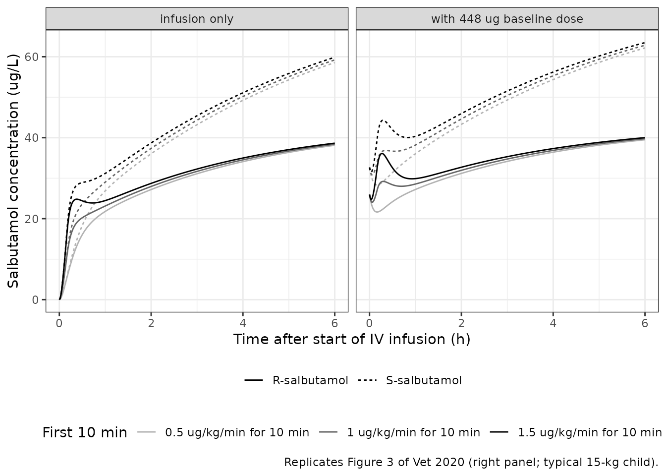

at15 <- sim_fig3 |>
  dplyr::filter(abs(time - 0.25) < 1e-8, ld_rate %in% c(0.5, 1.5)) |>
  dplyr::select(ld_rate, baseline, Cc_r_enant, Cc_s_enant)
cell <- function(d, ld, base, col) {
  v <- d[[col]][d$ld_rate == ld & d$baseline == base]
  if (length(v) != 1L) stop("no unique row for ld_rate ", ld, ", baseline ", base)
  v
}
chk15 <- tibble::tibble(
  Quantity = c(
    "R, no loading dose", "S, no loading dose",
    "R, 1.5 ug/kg/min loading dose", "S, 1.5 ug/kg/min loading dose",
    "R, loading-dose increment", "S, loading-dose increment"
  ),
  Model = c(
    cell(at15, 0.5, TRUE, "Cc_r_enant"), cell(at15, 0.5, TRUE, "Cc_s_enant"),
    cell(at15, 1.5, TRUE, "Cc_r_enant"), cell(at15, 1.5, TRUE, "Cc_s_enant"),
    cell(at15, 1.5, FALSE, "Cc_r_enant") - cell(at15, 0.5, FALSE, "Cc_r_enant"),
    cell(at15, 1.5, FALSE, "Cc_s_enant") - cell(at15, 0.5, FALSE, "Cc_s_enant")
  ),
  Published = c(22.2, 29.2, 36.7, 45.7, 36.7 - 22.2, 45.7 - 29.2)
) |>
  dplyr::mutate(`Difference (%)` = 100 * (Model / Published - 1))
knitr::kable(
  chk15,
  digits = 1,
  caption = "Concentrations 15 min after the start of the infusion (ug/L), model vs Vet 2020 Section 3.4. The increment rows are the 1.5 ug/kg/min minus the no-loading-dose value and do not depend on the baseline dose."
)

Concentrations 15 min after the start of the infusion (ug/L), model vs Vet 2020 Section 3.4. The increment rows are the 1.5 ug/kg/min minus the no-loading-dose value and do not depend on the baseline dose.
Quantity	Model	Published	Difference (%)
R, no loading dose	22.0	22.2	-0.8
S, no loading dose	28.7	29.2	-1.6
R, 1.5 ug/kg/min loading dose	36.0	36.7	-1.8
S, 1.5 ug/kg/min loading dose	44.0	45.7	-3.8
R, loading-dose increment	14.0	14.5	-3.4
S, loading-dose increment	15.2	16.5	-7.7

The loading-dose increment at 15 min does not depend on how the baseline dose is handled, so it tests the disposition model on its own. The model gives 14.0 ug/L for R and 15.2 ug/L for S, against 14.5 and 16.5 in the paper (3 % and 8 % low). The four absolute 15-min values agree within 1-4 %, but the baseline dose timing was back-solved from those same values, so they are a consistency check and not an independent one.

# Deterministic typical-value solve: the only noise is the integrator.
# Increments: realised -3 % (R) and -8 % (S); a mis-transcribed CL, Vc, Q or
# split fraction moves them by tens of percent.
stopifnot(all(abs(chk15$`Difference (%)`[5:6]) < 12))
# Absolute values with the back-solved baseline: realised within 4 %.
stopifnot(all(abs(chk15$`Difference (%)`[1:4]) < 6))

# Figure 3 at 6 h (read from the figure): R about 40, S about 63-64 ug/L.
at6 <- sim_fig3 |> dplyr::filter(abs(time - 6) < 1e-8, baseline)
stopifnot(
  all(abs(at6$Cc_r_enant / 40 - 1) < 0.08),
  all(abs(at6$Cc_s_enant / 63.5 - 1) < 0.08)
)
at6 |> dplyr::select(ld_rate, Cc_r_enant, Cc_s_enant) |> knitr::kable(digits = 1, caption = "Concentrations at 6 h (ug/L); Figure 3 shows about 40 (R) and 63-64 (S).")

Concentrations at 6 h (ug/L); Figure 3 shows about 40 (R) and 63-64 (S).
ld_rate	Cc_r_enant	Cc_s_enant
0.5	39.5	62.2
1.0	39.8	62.8
1.5	40.0	63.5

Virtual cohort and stochastic simulation

The original data are not public. The cohort below has 200 children whose weights follow a log-normal distribution with median 18 kg, truncated to the observed 7.8-70 kg range (Table 1). Each child gets a 24-h infusion of 1 ug/kg/min, close to the median rate (0.96 ug/kg/min) and median duration (22.5 h) in the study. Each child also gets an individual baseline dose, 448 ug * exp(eta) with eta drawn from N(0, log(1 + 0.99^2)) (Table 2 IPV 99 %), given into depot 0.4 h before the infusion as in the Figure 3 replication.

# set.seed() seeds R's RNG (weights and baseline-dose etas below), not
# rxode2's; the simulated etas differ across thread counts, so every check
# downstream is on medians.
set.seed(20200201)
n_sub <- 200L
wt_draw <- numeric(0)
while (length(wt_draw) < n_sub) {
  w <- rlnorm(4L * n_sub, log(18), 0.55)
  wt_draw <- c(wt_draw, w[w >= 7.8 & w <= 70])
}
subj <- tibble::tibble(
  id = seq_len(n_sub),
  WT = round(wt_draw[seq_len(n_sub)], 1),
  baseline_ug = 448 * exp(rnorm(n_sub, 0, sqrt(log(1 + 0.99^2))))
)
obs_times <- c(0, 0.25, 0.5, 1, 2, 4, 6, 8, 12, 16, 20, 24)
ev_vpc <- dplyr::bind_rows(
  subj |> dplyr::transmute(id, WT, time = 0, amt = baseline_ug, rate = 0, evid = 1L, cmt = "depot", dvid = NA_integer_),
  subj |> dplyr::transmute(id, WT, time = 0.4, amt = 1 * WT * 60 * 24, rate = 1 * WT * 60, evid = 1L, cmt = "depot", dvid = NA_integer_),
  tidyr::expand_grid(subj |> dplyr::select(id, WT), time = 0.4 + obs_times) |>
    dplyr::mutate(amt = NA_real_, rate = NA_real_, evid = 0L, cmt = NA_character_, dvid = 1L)
) |>
  dplyr::arrange(id, time, dplyr::desc(evid))
summary(subj$WT)
#>    Min. 1st Qu.  Median    Mean 3rd Qu.    Max. 
#>    8.00   14.15   19.30   21.72   25.70   60.70

rxode2::rxSetSeed(20200201)
sim_vpc <- rxode2::rxSolve(mod, ev_vpc, keep = "WT", returnType = "data.frame") |>
  dplyr::mutate(time = time - 0.4)
stopifnot(!anyNA(sim_vpc$Cc_r_enant), !anyNA(sim_vpc$Cc_s_enant))

vpc <- sim_vpc |>
  tidyr::pivot_longer(c(Cc_r_enant, Cc_s_enant), names_to = "enantiomer", values_to = "Cc") |>
  dplyr::mutate(enantiomer = ifelse(enantiomer == "Cc_r_enant", "R-salbutamol", "S-salbutamol")) |>
  dplyr::group_by(time, enantiomer) |>
  dplyr::summarise(
    Q05 = quantile(Cc, 0.05), Q50 = median(Cc), Q95 = quantile(Cc, 0.95),
    .groups = "drop"
  )
ggplot(vpc, aes(time, Q50, fill = enantiomer, colour = enantiomer)) +
  geom_ribbon(aes(ymin = Q05, ymax = Q95), alpha = 0.2, colour = NA) +
  geom_line() +
  scale_y_log10() +
  labs(
    x = "Time after start of IV infusion (h)",
    y = "Concentration (ug/L)", colour = NULL, fill = NULL,
    caption = "Simulated 5th-95th percentiles and median, 1 ug/kg/min for 24 h, 200 virtual children."
  ) +
  theme_bw()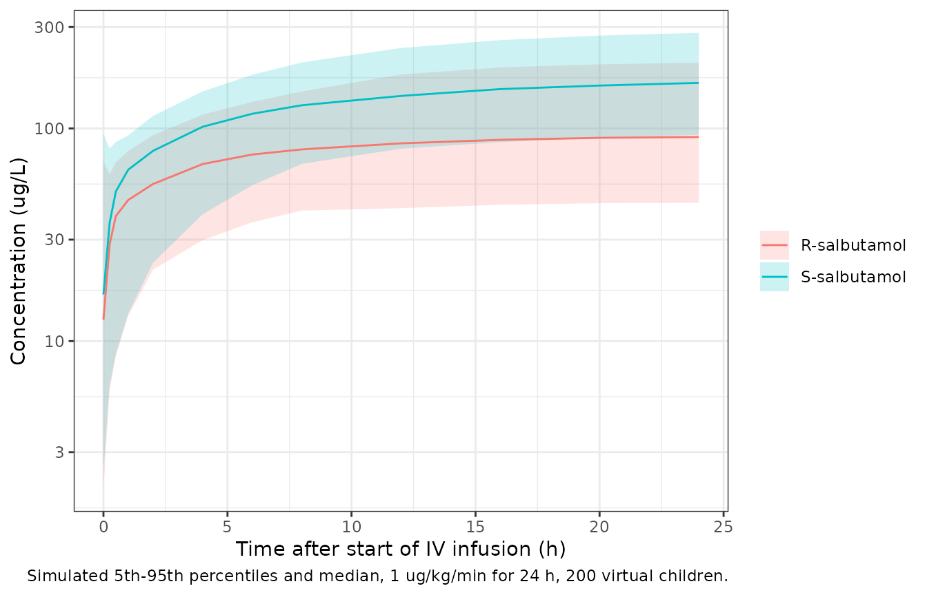

The paper reports the median concentration during the IV infusion as 66 ug/L for R-salbutamol (range 4-969) and 108 ug/L for S-salbutamol (range 19-1094) (Section 3.1). Those observations come from titrated infusion rates and from samples taken across the course of treatment, so they are only a rough reference. The simulated medians over 0.25-24 h are in the same range, and the S/R ratio is close to the observed 108/66 = 1.6.

med_iv <- sim_vpc |>
  dplyr::filter(time >= 0.25) |>
  dplyr::summarise(R = median(Cc_r_enant), S = median(Cc_s_enant))
knitr::kable(
  tibble::tibble(
    Statistic = c("Median R-salbutamol (ug/L)", "Median S-salbutamol (ug/L)", "S/R ratio of medians"),
    Simulated = c(med_iv$R, med_iv$S, med_iv$S / med_iv$R),
    Observed = c(66, 108, 108 / 66)
  ),
  digits = 2
)

Statistic	Simulated	Observed
Median R-salbutamol (ug/L)	64.78	66.00
Median S-salbutamol (ug/L)	104.55	108.00
S/R ratio of medians	1.61	1.64

# A factor-of-2 envelope: the observed medians come from a titrated regimen.
# The S/R ratio is set by CL_R / CL_S (1.85 at steady state) and is far
# tighter; a swapped or mistyped clearance takes it outside 1.2-2.4.
stopifnot(
  med_iv$R > 66 / 2, med_iv$R < 66 * 2,
  med_iv$S > 108 / 2, med_iv$S < 108 * 2,
  med_iv$S / med_iv$R > 1.2, med_iv$S / med_iv$R < 2.4
)

PKNCA validation

The paper reports no NCA. As an internal check, the cohort below receives a single IV loading dose of 10 or 15 ug/kg over 10 min (the bolus doses cited in the Discussion), with no baseline dose, and PKNCA computes Cmax, Tmax, AUC0-inf and half-life for each enantiomer. Each child’s AUC0-inf for an enantiomer should equal 0.5 * dose / CL for that enantiomer.

make_bolus_arm <- function(n, dose_ugkg, id_offset) {
  tibble::tibble(id = id_offset + seq_len(n), WT = sample(subj$WT, n, replace = TRUE)) |>
    dplyr::mutate(treatment = paste(dose_ugkg, "ug/kg over 10 min"), amt_total = dose_ugkg * WT)
}
set.seed(20200202)
arms <- dplyr::bind_rows(
  make_bolus_arm(100L, 10, 0L),
  make_bolus_arm(100L, 15, 100L)
)
nca_times <- c(0, 1 / 12, 1 / 6, 0.25, 0.5, 0.75, 1, 1.5, 2, 3, 4, 6, 8, 10, 12, 16, 24)
ev_nca <- dplyr::bind_rows(
  arms |> dplyr::transmute(id, WT, treatment, time = 0, amt = amt_total, rate = amt_total * 6, evid = 1L, cmt = "depot", dvid = NA_integer_),
  tidyr::expand_grid(arms |> dplyr::select(id, WT, treatment), time = nca_times) |>
    dplyr::mutate(amt = NA_real_, rate = NA_real_, evid = 0L, cmt = NA_character_, dvid = 1L)
) |>
  dplyr::arrange(id, time, dplyr::desc(evid))
stopifnot(!anyDuplicated(unique(ev_nca[, c("id", "time", "evid")])))

rxode2::rxSetSeed(20200202)
sim_nca <- rxode2::rxSolve(mod, ev_nca, keep = "treatment", returnType = "data.frame")
stopifnot(all(sim_nca$Cc_r_enant >= -1e-6 * max(sim_nca$Cc_r_enant)))
conc_long <- sim_nca |>
  dplyr::select(id, time, treatment, Cc_r_enant, Cc_s_enant) |>
  tidyr::pivot_longer(c(Cc_r_enant, Cc_s_enant), names_to = "analyte", values_to = "Cc") |>
  dplyr::filter(!is.na(Cc)) |>
  dplyr::mutate(Cc = pmax(Cc, 0), analyte = ifelse(analyte == "Cc_r_enant", "R", "S"))
conc_long <- dplyr::bind_rows(
  conc_long,
  conc_long |> dplyr::distinct(id, treatment, analyte) |> dplyr::mutate(time = 0, Cc = 0)
) |>
  dplyr::distinct(id, treatment, analyte, time, .keep_all = TRUE) |>
  dplyr::arrange(id, analyte, time)

conc_obj <- PKNCA::PKNCAconc(conc_long, Cc ~ time | treatment + id / analyte)
dose_df <- ev_nca |>
  dplyr::filter(evid == 1) |>
  dplyr::select(id, time, amt, treatment) |>
  dplyr::mutate(duration = 1 / 6)
dose_obj <- PKNCA::PKNCAdose(dose_df, amt ~ time | treatment + id, duration = "duration")
intervals <- data.frame(
  start = 0, end = Inf,
  cmax = TRUE, tmax = TRUE, aucinf.obs = TRUE, half.life = TRUE
)
nca_res <- PKNCA::pk.nca(PKNCA::PKNCAdata(conc_obj, dose_obj, intervals = intervals))
nca_tab <- as.data.frame(nca_res)
nca_tab |>
  dplyr::filter(PPTESTCD %in% c("cmax", "tmax", "aucinf.obs", "half.life")) |>
  dplyr::group_by(treatment, analyte, PPTESTCD) |>
  dplyr::summarise(median = median(PPORRES, na.rm = TRUE), .groups = "drop") |>
  tidyr::pivot_wider(names_from = PPTESTCD, values_from = median) |>
  dplyr::rename(
    "Dose" = treatment, "Enantiomer" = analyte,
    "Cmax (ug/L)" = cmax, "Tmax (h)" = tmax,
    "AUC0-inf (ug*h/L)" = aucinf.obs, "t1/2 (h)" = half.life
  ) |>
  knitr::kable(digits = 2, caption = "Simulated NCA (median across 100 children per dose and enantiomer).")

Simulated NCA (median across 100 children per dose and enantiomer).
Dose	Enantiomer	AUC0-inf (ug*h/L)	Cmax (ug/L)	t1/2 (h)	Tmax (h)
10 ug/kg over 10 min	R	15.08	12.05	3.01	0.25
10 ug/kg over 10 min	S	28.13	13.57	4.55	0.25
15 ug/kg over 10 min	R	22.73	20.86	2.73	0.25
15 ug/kg over 10 min	S	45.03	23.87	4.63	0.25

cl_ind <- sim_nca |>
  dplyr::distinct(id, cl_r_enant, cl_s_enant) |>
  tidyr::pivot_longer(c(cl_r_enant, cl_s_enant), names_to = "analyte", values_to = "cl") |>
  dplyr::mutate(analyte = ifelse(analyte == "cl_r_enant", "R", "S"))
auc_chk <- nca_tab |>
  dplyr::filter(PPTESTCD == "aucinf.obs") |>
  dplyr::left_join(cl_ind, by = c("id", "analyte")) |>
  dplyr::left_join(arms |> dplyr::select(id, amt_total), by = "id") |>
  dplyr::mutate(pct_diff = 100 * (PPORRES / (0.5 * amt_total / cl) - 1))
stopifnot(nrow(auc_chk) == 400L)
auc_chk |>
  dplyr::group_by(analyte) |>
  dplyr::summarise(
    `Median difference (%)` = median(pct_diff, na.rm = TRUE),
    `90th percentile of |difference| (%)` = quantile(abs(pct_diff), 0.9, na.rm = TRUE),
    .groups = "drop"
  ) |>
  dplyr::rename(Enantiomer = analyte) |>
  knitr::kable(digits = 2, caption = "PKNCA AUC0-inf vs 0.5 * dose / CL per child.")

PKNCA AUC0-inf vs 0.5 * dose / CL per child.
Enantiomer	Median difference (%)	90th percentile of \|difference\| (%)
R	-0.17	0.79
S	-0.10	0.54

# Trapezoid and tail-extrapolation error only; a wrong split fraction or
# a lost peripheral compartment moves the centre by far more than 5 %.
stopifnot(
  abs(median(auc_chk$pct_diff, na.rm = TRUE)) < 5,
  quantile(abs(auc_chk$pct_diff), 0.9, na.rm = TRUE) < 15
)

No published NCA values exist for comparison, so no side-by-side table is shown.

Assumptions and deviations

Baseline dose (prior inhalation) is not part of the model. Table 2 gives a fitted per-patient baseline dose of 448 ug (RSE 25 %, IPV 99 %), split equally between R- and S-salbutamol, that stands for salbutamol already in the body from inhalation. The paper does not state when it is given, which compartment receives it, or whether it is scaled by weight. The maintainers tested the simple readings for a 15-kg child against the printed 15-min values. A bolus into the dosing compartment at the start of the infusion gives zero concentration at time 0, against about 16 (R) and 23 (S) ug/L in Figure 3. A weight-scaled amount gives S-salbutamol 35 % low at 15 min. An unscaled bolus straight into the central compartments gives 81 ug/L at time 0, against “approximately 20”. So the model file holds only the disposition model, and the baseline dose is supplied as a dose record. For the simulations in this article the maintainers back-solved the timing: 448 ug, not weight-scaled, into depot 0.4 h before the infusion. This reproduces the printed 15-min values within 1-4 %, but the concentration at time 0 is about 26 (R) and 33 (S) ug/L, higher than the 16 and 23 in Figure 3. The 0.4-h lead time is the maintainers’ back-solve, not a value from the paper.
IPV scale. Table 2 reports IPV in % for an exponential model. It is read as a CV, omega^2 = log(1 + CV^2), which gives 2.19 for the 281 % on Vc. Reading it as sqrt(omega^2) * 100 would give 7.90 instead. The paper does not say which convention it used.
Residual error. The 0.351 in Table 2 is taken as the SD of an additive error on log-transformed concentrations, which is lnorm(0.351) here. Table 2 gives one value for both enantiomers, and nlmixr2 needs one residual parameter per endpoint, so the model carries it twice (expSd_r_enant, expSd_s_enant).
Shared Vc eta. The Table 2 footnote says Vc is identical for the two enantiomers. The single IPV on Vc is therefore one eta applied to both enantiomers’ central volume.
Virtual cohort. The weight distribution (log-normal, median 18 kg, truncated to 7.8-70 kg) and the 1 ug/kg/min for 24 h regimen are the maintainers’ approximation of Table 1. The paper did not report race or ethnicity.
No erratum or correction notice was found on Europe PMC (searched 2026-10-16).