Unbound teicoplanin (Fu 2022)
Source:vignettes/articles/Fu_2022_teicoplanin.Rmd
Fu_2022_teicoplanin.RmdModel and source
mod <- readModelDb("Fu_2022_teicoplanin")
ui <- rxode2::rxode(mod)
#> ℹ parameter labels from comments will be replaced by 'label()'- Citation: Fu W-Q, Tian T-T, Zhang M-X, Song H-T, Zhang L-L. Population pharmacokinetics and dosing optimization of unbound teicoplanin in Chinese adult patients. Front Pharmacol. 2022;13:1045895. doi:10.3389/fphar.2022.1045895
- Article: https://doi.org/10.3389/fphar.2022.1045895 (PMC9728581, open access)
- Supplement: Supplementary Table 1, “Simulation results for the recommended dosing regimen” (published with the article).
Fu 2022 is one of the few teicoplanin population models fitted to unbound concentrations: plasma was ultrafiltered at 37 C and the ultrafiltrate assayed by UPLC-MS/MS. A one-compartment model with first-order elimination fitted the 103 unbound concentrations from 72 Chinese adults; a two-compartment model did not improve the fit (dOFV -0.24) and was over-parameterised (condition number 1.16e7). The CKD-EPI estimated glomerular filtration rate (eGFR) on clearance and serum albumin on volume were the retained covariates:
-
CL (L/h) = 11.7 x (eGFR / 84)^0.476 x exp(eta_CL)(Results Eq 10) -
V (L) = 811 x (ALB / 32)^1.6 x exp(eta_V)(Results Eq 11)
Because the modelled state is unbound drug, 811 L is the apparent volume of unbound teicoplanin, about ten times the total-drug volume the same group reported (83.1 L); with 90-95% of teicoplanin bound to albumin, a lower albumin raises the unbound fraction and therefore shrinks the apparent unbound volume, which is the positive albumin exponent.
Population
The cohort was 72 adult inpatients (46 male, 26 female) treated with intravenous teicoplanin at the 900th Hospital of Joint Logistics Support Force, Fuzhou, during 2019 (Fu 2022 Table 1). Age was 69 +/- 20 years (range 18-99), weight 61.0 +/- 9.8 kg (40-85), serum creatinine 86.2 +/- 48.3 umol/L, eGFR 80.8 +/- 27.1 (17.4-134.0) and serum albumin 31.0 +/- 5.1 g/L (18.3-46.0). Most infections were pulmonary (58, 80.6%), followed by skin (6), pyemia (4), bacteraemia (3), abdominal (2), biliary tract (2) and liver abscess (1). Haemodialysis, continuous renal replacement therapy, disseminated intravascular coagulation and pregnancy were exclusions.
The standard regimen was 400 mg every 12 h for three doses, then 400 or 200 mg once daily, each as a 40-min infusion, but doses were at physician discretion (daily dose 50-1600 mg). Sampling was sparse (1-5 samples per patient, mostly troughs before the 4th and 6th doses). Observed unbound concentrations were 1.5 +/- 0.9 ug/mL (range 0.4-4.4).
The same information is available programmatically via
readModelDb("Fu_2022_teicoplanin")()$population.
Source trace
| Equation / parameter | Value | Source location |
|---|---|---|
lcl (unbound CL at eGFR 84) |
11.7 L/h | Table 2, thetaCL; Results Eq 10; Abstract |
lvc (unbound V at ALB 32 g/L) |
811 L | Table 2, thetaV; Results Eq 11; Abstract |
e_crcl_cl (eGFR exponent on CL) |
0.476 | Table 2, thetaeGFR; Eq 10 exponent |
e_alb_vc (albumin exponent on V) |
1.60 | Table 2, thetaALB; Eq 11 exponent (printed 1.6) |
etalcl |
0.386^2 = 0.149 | Table 2, etaCL = 38.6% |
etalvc |
0.537^2 = 0.288 | Table 2, etaV = 53.7% |
propSd |
0.183 | Table 2, eps1 = 18.3% |
addSd |
0.122 mg/L | Table 2, eps2 = 0.122 ug/mL |
cl <- exp(lcl + etalcl) * (CRCL / 84)^e_crcl_cl |
n/a | Eq 10; covariate form Methods Eq 7; exponential IIV Methods Eq 5 |
vc <- exp(lvc + etalvc) * (ALB / 32)^e_alb_vc |
n/a | Eq 11 |
| one-compartment, first-order elimination, IV infusion | n/a | Results, “Population pharmacokinetics modeling” (ADVAN1 TRANS2); Methods, 40-min infusion |
Cc ~ add(addSd) + prop(propSd) |
n/a | Methods Eq 6, Y = F x (1 + eps1) + eps2
|
| eGFR = CKD-EPI (creatinine, 2009) | n/a | Methods Eqs 1-4 |
ui$iniDf |>
  dplyr::select(name, est, fix, label) |>
  dplyr::rename(
    "Parameter" = name, "Estimate" = est,
    "Fixed" = fix, "Label" = label
  ) |>
knitr::kable(digits = 6, caption = "Packaged `ini()` block.")| Parameter | Estimate | Fixed | Label |
|---|---|---|---|
| lcl | 2.459589 | FALSE | Unbound clearance at eGFR = 84 (L/h) |
| lvc | 6.698268 | FALSE | Unbound volume of distribution at ALB = 32 g/L (L) |
| e_crcl_cl | 0.476000 | FALSE | Power exponent of eGFR on unbound CL (unitless) |
| e_alb_vc | 1.600000 | FALSE | Power exponent of serum albumin on unbound V (unitless) |
| propSd | 0.183000 | FALSE | Proportional residual error (fraction) |
| addSd | 0.122000 | FALSE | Additive residual error (mg/L) |
| etalcl | 0.148996 | FALSE | Fu 2022 Table 2: etaCL = 38.6% (RSE 16.5%; shrinkage 35%) -> 0.386^2 |
| etalvc | 0.288369 | FALSE | Fu 2022 Table 2: etaV = 53.7% (RSE 13.2%; shrinkage 31%) -> 0.537^2 |
Helpers
All simulations below use the dosing pattern of the paper: three loading doses every 12 h (0, 12, 24 h), then once-daily maintenance from 48 h, each over 40 min. The loading-dose trough is the 48 h concentration (before the first maintenance dose) and the maintenance trough the 96 h concentration.
dose_times <- c(0, 12, 24, 48, 72)
t_inf <- 40 / 60

regimen_events <- function(ids, ld, md, crcl, alb, obs_times) {
  doses <- expand.grid(id = ids, k = seq_along(dose_times))
  doses$time <- dose_times[doses$k]
  doses$amt <- ifelse(doses$k <= 3, ld, md)
  doses$evid <- 1L
  doses$dur <- t_inf
  obs <- expand.grid(id = ids, time = obs_times)
  obs$amt <- 0
  obs$evid <- 0L
  obs$dur <- 0
  dplyr::bind_rows(doses[, c("id", "time", "amt", "evid", "dur")], obs) |>
    dplyr::mutate(cmt = "central", CRCL = crcl, ALB = alb) |>
    dplyr::arrange(id, time, dplyr::desc(evid))
}
Structural check: ODE solution against the closed form
For a one-compartment model with constant-rate infusions the concentration is a sum of exponentials by superposition. Both sides use the same typical-value parameters, so the difference is integration error only.
crcl_ref <- 60
alb_ref <- 25
cl_ref <- 11.7 * (crcl_ref / 84)^0.476
v_ref <- 811 * (alb_ref / 32)^1.6
k_ref <- cl_ref / v_ref

closed_form <- function(t, ld, md) {
  amts <- c(rep(ld, 3), rep(md, 2))
  conc <- numeric(length(t))
  for (i in seq_along(dose_times)) {
    rate <- amts[i] / t_inf
    tt <- t - dose_times[i]
    during <- tt > 0 & tt <= t_inf
    after <- tt > t_inf
    conc[during] <- conc[during] + rate / cl_ref * (1 - exp(-k_ref * tt[during]))
    conc[after] <- conc[after] +
      rate / cl_ref * (1 - exp(-k_ref * t_inf)) * exp(-k_ref * (tt[after] - t_inf))
  }
  conc
}

cf_times <- c(0.5, 1, 6, 12, 24, 36, 48, 48.5, 72, 96, 120, 168)
cf_ev <- regimen_events(1L, 400, 400, crcl_ref, alb_ref, cf_times)
cf_sim <- rxode2::rxSolve(
  rxode2::zeroRe(mod), cf_ev, rtol = 1e-10, atol = 1e-12,
  returnType = "data.frame"
)
#> ℹ parameter labels from comments will be replaced by 'label()'
#> ℹ omega/sigma items treated as zero: 'etalcl', 'etalvc'
cf_cmp <- data.frame(time = cf_sim$time, ode = cf_sim$Cc) |>
  dplyr::mutate(
    closed = closed_form(time, 400, 400),
    rel_err = ode / closed - 1
  )
knitr::kable(
  cf_cmp |> dplyr::rename(
    "Time (h)" = time, "ODE (mg/L)" = ode,
    "Closed form (mg/L)" = closed, "Relative error" = rel_err
  ),
  digits = c(1, 4, 4, 12),
  caption = "400 mg x 3 q12h then 400 mg q24h; eGFR 60, albumin 25 g/L, typical subject."
)| Time (h) | ODE (mg/L) | Closed form (mg/L) | Relative error |
|---|---|---|---|
| 0.5 | 0.5466 | 0.5466 | 1.00e-12 |
| 1.0 | 0.7233 | 0.7233 | -9.60e-11 |
| 6.0 | 0.6602 | 0.6602 | -8.90e-11 |
| 12.0 | 0.5917 | 0.5917 | -9.50e-11 |
| 24.0 | 1.0671 | 1.0671 | -8.30e-11 |
| 36.0 | 1.4490 | 1.4490 | -6.20e-11 |
| 48.0 | 1.1641 | 1.1641 | -1.14e-10 |
| 48.5 | 1.7001 | 1.7001 | -1.60e-11 |
| 72.0 | 1.2267 | 1.2267 | -1.01e-10 |
| 96.0 | 1.2671 | 1.2671 | -8.10e-11 |
| 120.0 | 0.8178 | 0.8178 | -4.30e-11 |
| 168.0 | 0.3407 | 0.3407 | -8.50e-11 |
Typical-value PKNCA validation across covariate strata
A single 400 mg infusion is simulated for the typical subject at
several eGFR and albumin strata (the “treatment” group), sampled densely
to 30 days. PKNCA then recovers clearance as
Dose / AUC0-inf and the terminal half-life, which must
agree with Eqs 10-11.
strata <- expand.grid(CRCL = c(20, 84, 130), ALB = c(15, 32, 40)) |>
  dplyr::mutate(id = dplyr::row_number(), treatment = sprintf("eGFR %g / ALB %g", CRCL, ALB))
nca_times <- c(0, 0.25, 0.5, t_inf, 1, 2, 4, 8, 12, 24, 48, 72, 96, 144, 192, 288, 384, 480, 600, 720)
nca_ev <- dplyr::bind_rows(
  strata |> dplyr::mutate(time = 0, amt = 400, evid = 1L, dur = t_inf),
  tidyr::crossing(strata, time = nca_times) |> dplyr::mutate(amt = 0, evid = 0L, dur = 0)
) |>
  dplyr::mutate(cmt = "central") |>
  dplyr::arrange(id, time, dplyr::desc(evid))
nca_sim <- rxode2::rxSolve(
  rxode2::zeroRe(mod), nca_ev, rtol = 1e-10, atol = 1e-12,
  returnType = "data.frame", keep = "treatment"
)
#> ℹ parameter labels from comments will be replaced by 'label()'
#> ℹ omega/sigma items treated as zero: 'etalcl', 'etalvc'
#> Warning: multi-subject simulation without without 'omega'
# The fastest stratum (half-life about 12 h) decays below the integrator's
# absolute tolerance by 720 h; drop that numerically-zero tail after the peak
# so the half-life fit does not follow integrator noise.
stopifnot(all(nca_sim$Cc >= -1e-6 * max(nca_sim$Cc, na.rm = TRUE), na.rm = TRUE))
nca_conc <- nca_sim |>
  dplyr::filter(!is.na(Cc)) |>
  dplyr::mutate(Cc = pmax(Cc, 0)) |>
  dplyr::group_by(id) |>
  dplyr::filter(time <= time[which.max(Cc)] | Cc >= 1e-6 * max(Cc)) |>
  dplyr::ungroup() |>
  dplyr::select(id, treatment, time, Cc)
nca_dose <- strata |> dplyr::mutate(time = 0, amt = 400)

pk_conc <- PKNCA::PKNCAconc(nca_conc, Cc ~ time | treatment + id)
pk_dose <- PKNCA::PKNCAdose(nca_dose, amt ~ time | treatment + id)
pk_int <- data.frame(start = 0, end = Inf, cmax = TRUE, aucinf.obs = TRUE, half.life = TRUE, cl.obs = TRUE)
nca_res <- PKNCA::pk.nca(PKNCA::PKNCAdata(pk_conc, pk_dose, intervals = pk_int))

nca_tab <- as.data.frame(nca_res) |>
  dplyr::filter(PPTESTCD %in% c("cl.obs", "half.life", "cmax")) |>
  dplyr::select(treatment, PPTESTCD, PPORRES) |>
  tidyr::pivot_wider(names_from = PPTESTCD, values_from = PPORRES) |>
  dplyr::left_join(strata, by = "treatment") |>
  dplyr::mutate(
    cl_eq = 11.7 * (CRCL / 84)^0.476,
    thalf_eq = log(2) * 811 * (ALB / 32)^1.6 / cl_eq
  )
nca_tab |>
  dplyr::select(treatment, cmax, cl.obs, cl_eq, half.life, thalf_eq) |>
  dplyr::rename(
    "Stratum" = treatment, "Cmax (mg/L)" = cmax,
    "PKNCA CL (L/h)" = cl.obs, "Eq 10 CL (L/h)" = cl_eq,
    "PKNCA t1/2 (h)" = half.life, "log(2) V / CL (h)" = thalf_eq
  ) |>
knitr::kable(digits = 2, caption = "PKNCA on typical-subject single 400 mg doses.")| Stratum | Cmax (mg/L) | PKNCA CL (L/h) | Eq 10 CL (L/h) | PKNCA t1/2 (h) | log(2) V / CL (h) |
|---|---|---|---|---|---|
| eGFR 130 / ALB 15 | 1.63 | 14.40 | 14.40 | 11.61 | 11.61 |
| eGFR 130 / ALB 32 | 0.49 | 14.40 | 14.40 | 39.03 | 39.03 |
| eGFR 130 / ALB 40 | 0.34 | 14.40 | 14.40 | 55.77 | 55.77 |
| eGFR 20 / ALB 15 | 1.64 | 5.91 | 5.91 | 28.30 | 28.30 |
| eGFR 20 / ALB 32 | 0.49 | 5.91 | 5.91 | 95.13 | 95.13 |
| eGFR 20 / ALB 40 | 0.34 | 5.91 | 5.91 | 135.95 | 135.95 |
| eGFR 84 / ALB 15 | 1.63 | 11.70 | 11.70 | 14.29 | 14.29 |
| eGFR 84 / ALB 32 | 0.49 | 11.70 | 11.70 | 48.05 | 48.05 |
| eGFR 84 / ALB 40 | 0.34 | 11.70 | 11.70 | 68.66 | 68.66 |
# Deterministic solves; the residual is the trapezoid/extrapolation error of a
# 20-point grid, well under 2% for CL and 1% for the half-life fit.
stopifnot(
  max(abs(nca_tab$cl.obs / nca_tab$cl_eq - 1)) < 0.02,
  max(abs(nca_tab$half.life / nca_tab$thalf_eq - 1)) < 0.01
)
The unbound half-life spans roughly 12 h (eGFR 130, albumin 15 g/L) to more than 100 h (eGFR 20, albumin 40 g/L), which is why both covariates move the loading and maintenance doses the paper recommends.
Virtual cohort and standard-regimen profile
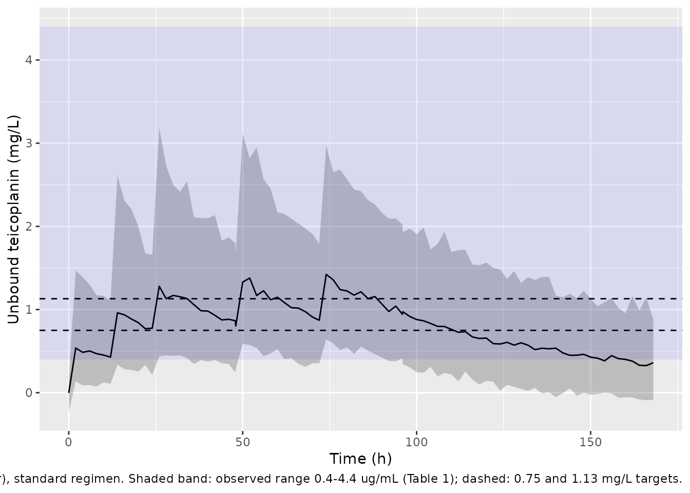
A virtual cohort of 200 adults draws eGFR and albumin independently from normal distributions with the Table 1 mean and SD, truncated to the observed ranges. Each receives the standard regimen (400 mg x 3 q12h, then 400 mg q24h).
rxode2::rxSetSeed(20221123)
n_cohort <- 200
cohort <- data.frame(
  id = seq_len(n_cohort),
  CRCL = pmin(pmax(stats::rnorm(n_cohort, 80.8, 27.1), 17.4), 134.0),
  ALB = pmin(pmax(stats::rnorm(n_cohort, 31.0, 5.1), 18.3), 46.0)
)
prof_times <- sort(unique(c(seq(0, 168, by = 2), 47.9, 95.9)))
prof_ev <- regimen_events(cohort$id, 400, 400, NA_real_, NA_real_, prof_times) |>
  dplyr::select(-CRCL, -ALB) |>
  dplyr::left_join(cohort, by = "id")
prof_sim <- rxode2::rxSolve(mod, prof_ev, returnType = "data.frame")
#> ℹ parameter labels from comments will be replaced by 'label()'

prof_sim |>
  dplyr::group_by(time) |>
  dplyr::summarise(
    q05 = stats::quantile(sim, 0.05), q50 = stats::median(sim), q95 = stats::quantile(sim, 0.95),
    .groups = "drop"
  ) |>
  ggplot(aes(time, q50)) +
  geom_ribbon(aes(ymin = q05, ymax = q95), alpha = 0.25) +
  geom_line() +
  geom_hline(yintercept = c(0.75, 1.13), linetype = "dashed") +
  annotate("rect", xmin = -Inf, xmax = Inf, ymin = 0.4, ymax = 4.4, alpha = 0.08, fill = "blue") +
  labs(
    x = "Time (h)", y = "Unbound teicoplanin (mg/L)",
    caption = paste(
      "Median and 90% prediction interval (with residual error), standard regimen.",
      "Shaded band: observed range 0.4-4.4 ug/mL (Table 1); dashed: 0.75 and 1.13 mg/L targets."
    )
  )
troughs <- prof_sim |>
  dplyr::filter(time %in% c(47.9, 95.9)) |>
  dplyr::group_by(time) |>
  dplyr::summarise(median = stats::median(Cc), q05 = stats::quantile(Cc, 0.05),
                   q95 = stats::quantile(Cc, 0.95), .groups = "drop")
knitr::kable(
  troughs |> dplyr::rename("Time (h)" = time, "Median (mg/L)" = median, "5th pct" = q05, "95th pct" = q95),
  digits = 2, caption = "Simulated unbound troughs before the 4th and 6th doses (standard regimen)."
)| Time (h) | Median (mg/L) | 5th pct | 95th pct |
|---|---|---|---|
| 47.9 | 0.85 | 0.38 | 1.55 |
| 95.9 | 0.96 | 0.38 | 1.93 |
# The sampled troughs in the study (before the 4th and 6th doses) averaged
# 1.5 ug/mL; a wrong volume unit or a total-vs-unbound mix-up moves the median
# trough by an order of magnitude.
stopifnot(all(troughs$median > 0.5 & troughs$median < 3))
The median simulated standard-regimen trough (0.85 mg/L at 48 h) lies inside the observed range of 0.4-4.4 ug/mL and below the observed mean of 1.5 ug/mL. That is the expected direction: doses were at physician discretion (up to 1600 mg/day), so many patients received more than the standard regimen, and not every sample was a trough.
Replicating Supplementary Table 1 and Table 3
The paper’s Monte Carlo simulations (n = 1000 per scenario) fix eGFR and albumin at six levels each and report, for each cell and target, the lowest loading dose and maintenance dose reaching PTA >= 80%, with the achieved PTA (Supplementary Table 1) and the probability of an unbound trough >= 4.5 mg/L at 96 h (Table 3, in brackets). Each regimen-cell is re-simulated here with 200 subjects using between-subject variability only (the residual error is a measurement model and is not part of a PTA).
supp <- utils::read.table(header = TRUE, text = "
egfr alb ld1 pta1 md2 pta2 ld3 pta3 md4 pta4
20 15 400 96.2 400 94.3 400 89.5 400 83.2
20 20 400 97.4 200 90.2 400 84.5 400 88
20 25 400 94.7 200 90.6 600 94.3 200 83.7
20 30 400 87.1 200 88.4 600 87.4 200 82.3
20 35 600 93.4 200 93.6 800 88.7 200 86.3
20 40 600 88.6 200 91.4 800 82 200 81.7
30 15 400 90.7 400 86.7 600 92 600 83.9
30 20 400 95.7 400 94 600 95.2 400 86.9
30 25 400 92 200 81.8 600 90.5 400 88.7
30 30 400 80.3 200 80.3 600 83.4 400 86.3
30 35 600 92.3 200 90.3 800 88.6 400 90.5
30 40 600 85.8 200 85.6 1000 91.7 200 85
45 15 400 80.3 400 80.7 600 82.7 600 83.5
45 20 400 89.9 400 88.4 600 88.4 600 85.7
45 25 400 87.6 400 90.2 600 85.4 600 88.9
45 30 600 96 200 85.3 800 93.3 400 86.6
45 35 600 91.4 200 81.1 800 84.7 400 82.1
45 40 600 82.8 200 80.7 1000 88.7 400 87.9
60 15 600 86.5 600 80.1 800 82.3 800 80.2
60 20 400 82.8 400 80.7 600 81.1 600 80.1
60 25 400 80.7 400 84.1 800 93.6 600 86.7
60 30 600 95.3 400 91.5 800 90.4 600 88.6
60 35 600 89.7 400 91.2 800 85.1 600 88.5
60 40 600 83.5 400 88.2 1000 87.3 400 85
90 15 800 83.8 800 80.3 1000 80.8 1000 80.2
90 20 600 86.9 600 81.3 800 85.1 800 72.6
90 25 600 93.5 600 88.6 800 87.9 800 83.9
90 30 600 91 400 80.2 800 86.6 600 80.5
90 35 600 85.8 400 84 1000 91.9 600 85.6
90 40 800 91.8 400 89.8 1000 86.5 600 82.7
130 15 1000 80.3 1000 80.2 1200 80.8 1200 80.2
130 20 800 87.9 800 80.7 1000 81.5 1000 82.2
130 25 600 84.8 600 80.3 1000 87.9 800 83.3
130 30 600 84.8 600 84.2 1000 90.5 800 83.4
130 35 600 80.5 600 86.8 1000 87.1 800 83.1
130 40 800 90.9 400 80.8 1000 80.1 800 82.9
")
# Table 3 bracketed values, P(unbound trough >= 4.5 mg/L at 96 h) in %, in the
# same row order (eGFR outer, albumin inner) for each target.
tox_075 <- c(1.7, 0, 0, 0, 0, 0, 0.4, 0, 0, 0, 0, 0, 0.1, 0, 0, 0, 0, 0,
             0.8, 0, 0, 0, 0, 0, 1.7, 0, 0, 0, 0, 0, 1.7, 0.4, 0, 0, 0, 0)
tox_113 <- c(1.7, 0.5, 0.2, 0.2, 0.3, 0.4, 5.3, 0.7, 0.1, 0.1, 0.4, 0, 2.6, 1.5, 0.4, 0.4, 0, 0.2,
             4.6, 0.7, 1.0, 0.2, 0.4, 0.1, 4.6, 1.6, 0.9, 0.2, 0.2, 0.1, 4.7, 0.2, 0.4, 0, 0, 0)

pta_regs <- dplyr::bind_rows(
  supp |> dplyr::transmute(egfr, alb, target = 0.75, ld = ld1, md = md2,
                           pta_ld = pta1, pta_md = pta2, tox = tox_075),
  supp |> dplyr::transmute(egfr, alb, target = 1.13, ld = ld3, md = md4,
                           pta_ld = pta3, pta_md = pta4, tox = tox_113)
) |>
  dplyr::mutate(arm = dplyr::row_number())

n_arm <- 200
pta_events <- function(regs) {
  dplyr::bind_rows(lapply(seq_len(nrow(regs)), function(i) {
    ids <- (i - 1) * n_arm + seq_len(n_arm)
    regimen_events(ids, regs$ld[i], regs$md[i], regs$egfr[i], regs$alb[i], c(48, 96))
  }))
}
pta_ev <- pta_events(pta_regs)

summarise_pta <- function(sim, regs) {
  sim |>
    dplyr::mutate(arm = (id - 1) %/% n_arm + 1) |>
    dplyr::left_join(regs |> dplyr::select(arm, target), by = "arm") |>
    dplyr::group_by(arm) |>
    dplyr::summarise(
      sim_ld = 100 * mean(Cc[time == 48] >= target[1]),
      sim_md = 100 * mean(Cc[time == 96] >= target[1]),
      sim_tox = 100 * mean(Cc[time == 96] >= 4.5),
      .groups = "drop"
    ) |>
    dplyr::left_join(regs, by = "arm")
}

rxode2::rxSetSeed(1045895)
pta_sim <- rxode2::rxSolve(mod, pta_ev, returnType = "data.frame")
#> [====|====|====|====|====|====|====|====|====|====] 0:00:01
pta_res <- summarise_pta(pta_sim, pta_regs)

pta_res |>
  dplyr::transmute(
    target, egfr, alb, regimen = paste0(ld, "/", md),
    pta_ld, sim_ld, pta_md, sim_md, tox, sim_tox
  ) |>
  dplyr::rename(
    "Target (mg/L)" = target, "eGFR" = egfr, "ALB (g/L)" = alb,
    "LD/MD (mg)" = regimen,
    "PTA 48 h, paper (%)" = pta_ld, "PTA 48 h, sim (%)" = sim_ld,
    "PTA 96 h, paper (%)" = pta_md, "PTA 96 h, sim (%)" = sim_md,
    "P(>=4.5) 96 h, paper (%)" = tox, "P(>=4.5) 96 h, sim (%)" = sim_tox
  ) |>
knitr::kable(digits = 1, caption = "Supplementary Table 1 and Table 3 against the packaged model (200 subjects per cell).")| Target (mg/L) | eGFR | ALB (g/L) | LD/MD (mg) | PTA 48 h, paper (%) | PTA 48 h, sim (%) | PTA 96 h, paper (%) | PTA 96 h, sim (%) | P(>=4.5) 96 h, paper (%) | P(>=4.5) 96 h, sim (%) |
|---|---|---|---|---|---|---|---|---|---|
| 0.8 | 20 | 15 | 400/400 | 96.2 | 98.0 | 94.3 | 95.0 | 1.7 | 3.0 |
| 0.8 | 20 | 20 | 400/200 | 97.4 | 96.5 | 90.2 | 82.0 | 0.0 | 0.0 |
| 0.8 | 20 | 25 | 400/200 | 94.7 | 97.5 | 90.6 | 88.0 | 0.0 | 0.0 |
| 0.8 | 20 | 30 | 400/200 | 87.1 | 84.0 | 88.4 | 85.0 | 0.0 | 0.0 |
| 0.8 | 20 | 35 | 600/200 | 93.4 | 93.5 | 93.6 | 92.0 | 0.0 | 0.0 |
| 0.8 | 20 | 40 | 600/200 | 88.6 | 88.0 | 91.4 | 90.0 | 0.0 | 0.0 |
| 0.8 | 30 | 15 | 400/400 | 90.7 | 89.0 | 86.7 | 84.5 | 0.4 | 0.0 |
| 0.8 | 30 | 20 | 400/400 | 95.7 | 95.5 | 94.0 | 90.5 | 0.0 | 0.0 |
| 0.8 | 30 | 25 | 400/200 | 92.0 | 93.0 | 81.8 | 80.0 | 0.0 | 0.0 |
| 0.8 | 30 | 30 | 400/200 | 80.3 | 83.0 | 80.3 | 79.0 | 0.0 | 0.0 |
| 0.8 | 30 | 35 | 600/200 | 92.3 | 92.0 | 90.3 | 90.5 | 0.0 | 0.0 |
| 0.8 | 30 | 40 | 600/200 | 85.8 | 84.5 | 85.6 | 84.0 | 0.0 | 0.0 |
| 0.8 | 45 | 15 | 400/400 | 80.3 | 87.0 | 80.7 | 78.5 | 0.1 | 0.5 |
| 0.8 | 45 | 20 | 400/400 | 89.9 | 90.0 | 88.4 | 85.5 | 0.0 | 0.0 |
| 0.8 | 45 | 25 | 400/400 | 87.6 | 83.0 | 90.2 | 88.0 | 0.0 | 0.0 |
| 0.8 | 45 | 30 | 600/200 | 96.0 | 94.5 | 85.3 | 84.5 | 0.0 | 0.0 |
| 0.8 | 45 | 35 | 600/200 | 91.4 | 93.5 | 81.1 | 81.0 | 0.0 | 0.0 |
| 0.8 | 45 | 40 | 600/200 | 82.8 | 86.0 | 80.7 | 79.0 | 0.0 | 0.0 |
| 0.8 | 60 | 15 | 600/600 | 86.5 | 85.0 | 80.1 | 74.5 | 0.8 | 0.0 |
| 0.8 | 60 | 20 | 400/400 | 82.8 | 82.0 | 80.7 | 77.0 | 0.0 | 0.0 |
| 0.8 | 60 | 25 | 400/400 | 80.7 | 87.5 | 84.1 | 85.5 | 0.0 | 0.0 |
| 0.8 | 60 | 30 | 600/400 | 95.3 | 93.0 | 91.5 | 90.0 | 0.0 | 0.0 |
| 0.8 | 60 | 35 | 600/400 | 89.7 | 90.0 | 91.2 | 90.5 | 0.0 | 0.0 |
| 0.8 | 60 | 40 | 600/400 | 83.5 | 81.0 | 88.2 | 89.0 | 0.0 | 0.0 |
| 0.8 | 90 | 15 | 800/800 | 83.8 | 87.0 | 80.3 | 82.5 | 1.7 | 1.5 |
| 0.8 | 90 | 20 | 600/600 | 86.9 | 89.0 | 81.3 | 80.5 | 0.0 | 0.0 |
| 0.8 | 90 | 25 | 600/600 | 93.5 | 92.0 | 88.6 | 91.0 | 0.0 | 0.0 |
| 0.8 | 90 | 30 | 600/400 | 91.0 | 89.5 | 80.2 | 82.5 | 0.0 | 0.0 |
| 0.8 | 90 | 35 | 600/400 | 85.8 | 88.0 | 84.0 | 85.0 | 0.0 | 0.0 |
| 0.8 | 90 | 40 | 800/400 | 91.8 | 93.5 | 89.8 | 91.5 | 0.0 | 0.0 |
| 0.8 | 130 | 15 | 1000/1000 | 80.3 | 82.5 | 80.2 | 77.0 | 1.7 | 2.0 |
| 0.8 | 130 | 20 | 800/800 | 87.9 | 89.5 | 80.7 | 83.5 | 0.4 | 0.0 |
| 0.8 | 130 | 25 | 600/600 | 84.8 | 80.0 | 80.3 | 75.0 | 0.0 | 0.0 |
| 0.8 | 130 | 30 | 600/600 | 84.8 | 83.5 | 84.2 | 85.0 | 0.0 | 0.0 |
| 0.8 | 130 | 35 | 600/600 | 80.5 | 78.0 | 86.8 | 87.5 | 0.0 | 0.0 |
| 0.8 | 130 | 40 | 800/400 | 90.9 | 89.5 | 80.8 | 82.0 | 0.0 | 0.0 |
| 1.1 | 20 | 15 | 400/400 | 89.5 | 89.5 | 83.2 | 83.5 | 1.7 | 1.0 |
| 1.1 | 20 | 20 | 400/400 | 84.5 | 85.0 | 88.0 | 87.0 | 0.5 | 1.0 |
| 1.1 | 20 | 25 | 600/200 | 94.3 | 95.5 | 83.7 | 84.5 | 0.2 | 0.5 |
| 1.1 | 20 | 30 | 600/200 | 87.4 | 90.5 | 82.3 | 80.5 | 0.2 | 0.0 |
| 1.1 | 20 | 35 | 800/200 | 88.7 | 89.0 | 86.3 | 88.5 | 0.3 | 0.0 |
| 1.1 | 20 | 40 | 800/200 | 82.0 | 77.0 | 81.7 | 77.5 | 0.4 | 0.0 |
| 1.1 | 30 | 15 | 600/600 | 92.0 | 93.5 | 83.9 | 85.5 | 5.3 | 3.5 |
| 1.1 | 30 | 20 | 600/400 | 95.2 | 94.5 | 86.9 | 85.0 | 0.7 | 1.0 |
| 1.1 | 30 | 25 | 600/400 | 90.5 | 91.0 | 88.7 | 85.5 | 0.1 | 0.0 |
| 1.1 | 30 | 30 | 600/400 | 83.4 | 86.0 | 86.3 | 91.0 | 0.1 | 0.5 |
| 1.1 | 30 | 35 | 800/400 | 88.6 | 86.5 | 90.5 | 87.5 | 0.4 | 0.0 |
| 1.1 | 30 | 40 | 1000/200 | 91.7 | 88.5 | 85.0 | 85.0 | 0.0 | 0.0 |
| 1.1 | 45 | 15 | 600/600 | 82.7 | 81.5 | 83.5 | 71.5 | 2.6 | 2.5 |
| 1.1 | 45 | 20 | 600/600 | 88.4 | 87.5 | 85.7 | 86.0 | 1.5 | 2.0 |
| 1.1 | 45 | 25 | 600/600 | 85.4 | 84.0 | 88.9 | 88.5 | 0.4 | 0.0 |
| 1.1 | 45 | 30 | 800/400 | 93.3 | 91.5 | 86.6 | 85.5 | 0.4 | 0.0 |
| 1.1 | 45 | 35 | 800/400 | 84.7 | 87.5 | 82.1 | 87.0 | 0.0 | 0.0 |
| 1.1 | 45 | 40 | 1000/400 | 88.7 | 88.0 | 87.9 | 87.0 | 0.2 | 0.5 |
| 1.1 | 60 | 15 | 800/800 | 82.3 | 80.5 | 80.2 | 74.5 | 4.6 | 4.0 |
| 1.1 | 60 | 20 | 600/600 | 81.1 | 82.5 | 80.1 | 78.5 | 0.7 | 0.5 |
| 1.1 | 60 | 25 | 800/600 | 93.6 | 95.5 | 86.7 | 90.5 | 1.0 | 1.0 |
| 1.1 | 60 | 30 | 800/600 | 90.4 | 89.5 | 88.6 | 90.5 | 0.2 | 0.0 |
| 1.1 | 60 | 35 | 800/600 | 85.1 | 86.0 | 88.5 | 91.0 | 0.4 | 0.5 |
| 1.1 | 60 | 40 | 1000/400 | 87.3 | 88.5 | 85.0 | 84.5 | 0.1 | 0.0 |
| 1.1 | 90 | 15 | 1000/1000 | 80.8 | 77.0 | 80.2 | 69.5 | 4.6 | 8.0 |
| 1.1 | 90 | 20 | 800/800 | 85.1 | 82.0 | 72.6 | 73.0 | 1.6 | 1.0 |
| 1.1 | 90 | 25 | 800/800 | 87.9 | 87.5 | 83.9 | 82.0 | 0.9 | 0.5 |
| 1.1 | 90 | 30 | 800/600 | 86.6 | 86.5 | 80.5 | 81.5 | 0.2 | 0.5 |
| 1.1 | 90 | 35 | 1000/600 | 91.9 | 89.5 | 85.6 | 83.0 | 0.2 | 0.0 |
| 1.1 | 90 | 40 | 1000/600 | 86.5 | 84.5 | 82.7 | 81.5 | 0.1 | 0.0 |
| 1.1 | 130 | 15 | 1200/1200 | 80.8 | 68.0 | 80.2 | 59.5 | 4.7 | 6.0 |
| 1.1 | 130 | 20 | 1000/1000 | 81.5 | 84.0 | 82.2 | 73.0 | 0.2 | 1.5 |
| 1.1 | 130 | 25 | 1000/800 | 87.9 | 91.0 | 83.3 | 79.0 | 0.4 | 1.0 |
| 1.1 | 130 | 30 | 1000/800 | 90.5 | 89.0 | 83.4 | 82.0 | 0.0 | 0.0 |
| 1.1 | 130 | 35 | 1000/800 | 87.1 | 85.5 | 83.1 | 84.5 | 0.0 | 0.5 |
| 1.1 | 130 | 40 | 1000/800 | 80.1 | 82.5 | 82.9 | 86.5 | 0.0 | 0.0 |
d_all <- c(pta_res$sim_ld - pta_res$pta_ld, pta_res$sim_md - pta_res$pta_md)
pta_summary <- c(
  median_diff = stats::median(d_all),
  q75_abs_diff = unname(stats::quantile(abs(d_all), 0.75)),
  mean_tox_sim = mean(pta_res$sim_tox),
  mean_tox_paper = mean(pta_res$tox)
)
knitr::kable(t(pta_summary), digits = 2,
caption = "Simulated minus published PTA over 144 entries (percentage points), and mean toxicity probability.")| median_diff | q75_abs_diff | mean_tox_sim | mean_tox_paper |
|---|---|---|---|
| -0.75 | 2.8 | 0.62 | 0.58 |
# Monte Carlo SE of one cell is about 3 points at n = 200 (plus about 1 from
# the paper's own n = 1000), so the centre and the upper-quartile envelope
# carry the check. A mis-transcribed exponent or volume moves PTA by tens of
# points across the grid.
stopifnot(
  abs(pta_summary[["median_diff"]]) < 3,
  pta_summary[["q75_abs_diff"]] < 7,
  abs(pta_summary[["mean_tox_sim"]] - pta_summary[["mean_tox_paper"]]) < 1.5
)
pta_res |>
  tidyr::pivot_longer(c(sim_ld, sim_md), names_to = "when", values_to = "sim") |>
  dplyr::mutate(
    paper = ifelse(when == "sim_ld", pta_ld, pta_md),
    when = ifelse(when == "sim_ld", "Loading-dose trough, 48 h", "Maintenance trough, 96 h")
  ) |>
  ggplot(aes(paper, sim, colour = factor(egfr))) +
  geom_abline(linetype = "dashed") +
  geom_point() +
  facet_wrap(~when) +
  labs(x = "Published PTA (%)", y = "Simulated PTA (%)", colour = "eGFR",
       caption = "Supplementary Table 1 recommended regimens; 200 simulated subjects per point.")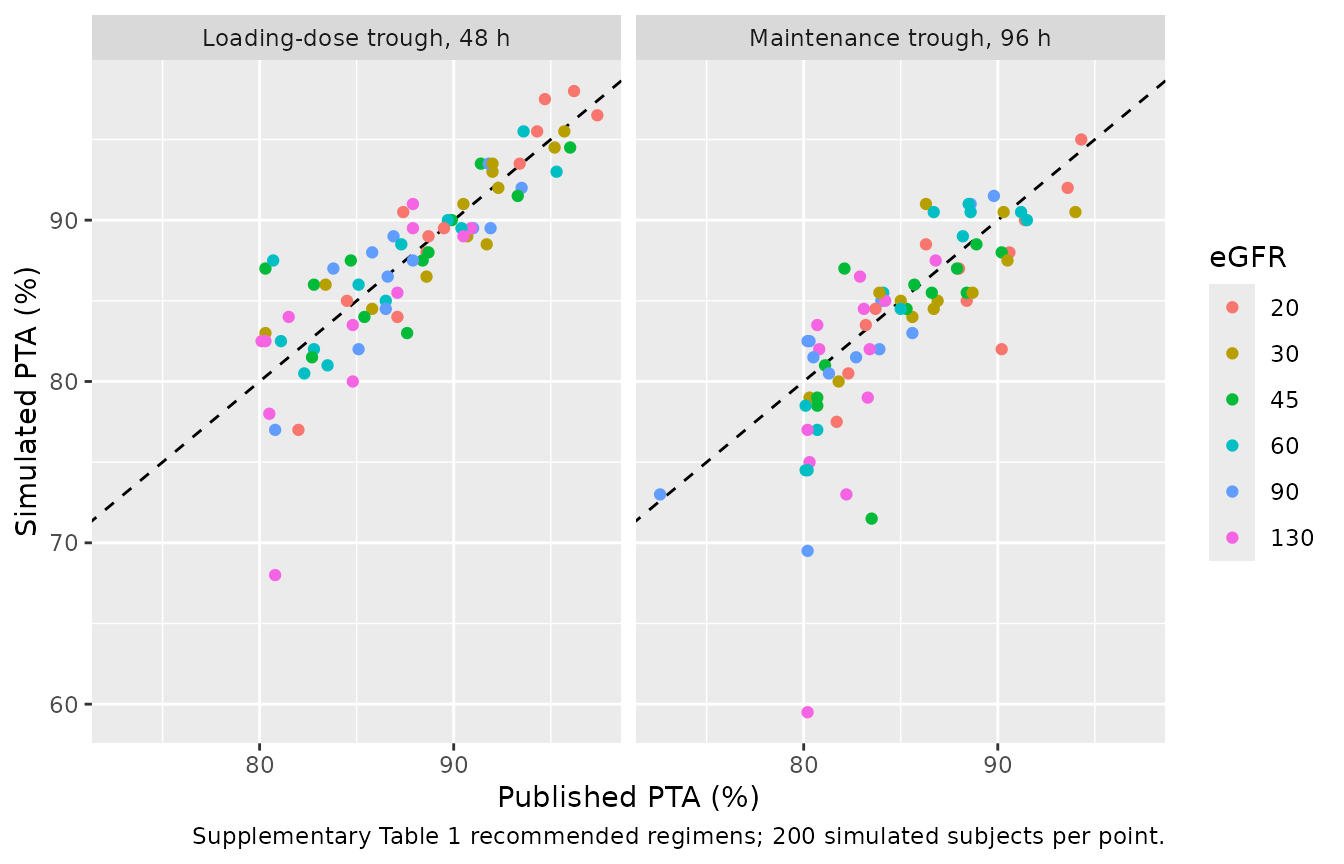
IIV scale
Table 2 prints the random effects as percentages (38.6% on CL, 53.7%
on V) without saying whether they are omega x 100 or a
log-normal CV. The two readings give variances of 0.149 / 0.288 and
0.139 / 0.253 respectively. The same 72 regimen-cells are simulated
under the CV reading for comparison.
mod_cv <- mod |> rxode2::ini(etalcl = log(1 + 0.386^2), etalvc = log(1 + 0.537^2))
#> ℹ parameter labels from comments will be replaced by 'label()'
#> ℹ change initial estimate of `etalcl` to `0.138888517572482`
#> ℹ change initial estimate of `etalvc` to `0.253377077334772`
rxode2::rxSetSeed(1045895)
pta_res_cv <- summarise_pta(rxode2::rxSolve(mod_cv, pta_ev, returnType = "data.frame"), pta_regs)
#> [====|====|====|====|====|====|====|====|====|====] 0:00:01
d_cv <- c(pta_res_cv$sim_ld - pta_res_cv$pta_ld, pta_res_cv$sim_md - pta_res_cv$pta_md)
knitr::kable(
  data.frame(
    reading = c("omega x 100 (packaged)", "log-normal CV"),
    median_diff = c(stats::median(d_all), stats::median(d_cv))
  ) |>
    dplyr::rename("IIV reading" = reading, "Median simulated - published PTA (points)" = median_diff),
  digits = 2
)| IIV reading | Median simulated - published PTA (points) |
|---|---|
| omega x 100 (packaged) | -0.75 |
| log-normal CV | 0.95 |
With 200 subjects per cell the median differences are -0.75 points
(omega x 100) and +0.95 points (CV); the median over 144
entries has a Monte Carlo standard error of roughly half a point at this
size. At 1000 subjects per cell (the paper’s own size) the maintainers
measured +0.05 points for the omega x 100 reading and +1.35
points for the CV reading, so the model ships the former. The two
readings differ by only 7-12% in variance, so the choice matters little
for simulation use.
Replicating Figure 3
Figure 3 plots PTA at 48 h against eGFR for loading doses of 400-1200 mg (q12h x 3), one panel per albumin level. Only the loading doses reach the 48 h trough, so the maintenance dose is irrelevant here.
fig3_regs <- tidyr::crossing(
  egfr = c(20, 30, 45, 60, 90, 130), alb = c(15, 20, 25, 30, 35, 40),
  ld = c(400, 600, 800, 1000, 1200)
) |>
  dplyr::mutate(md = 0, target = NA_real_, arm = dplyr::row_number())
fig3_ev <- pta_events(fig3_regs) |>
  dplyr::filter(!(evid == 1L & time >= 48), !(evid == 0L & time == 96))
rxode2::rxSetSeed(3)
fig3_sim <- rxode2::rxSolve(mod, fig3_ev, returnType = "data.frame") |>
  dplyr::mutate(arm = (id - 1) %/% n_arm + 1) |>
  dplyr::left_join(fig3_regs |> dplyr::select(arm, egfr, alb, ld), by = "arm")
#> [====|====|====|====|====|====|====|====|====|====] 0:00:01
fig3 <- fig3_sim |>
  dplyr::group_by(egfr, alb, ld) |>
  dplyr::summarise(`0.75 mg/L` = 100 * mean(Cc >= 0.75), `1.13 mg/L` = 100 * mean(Cc >= 1.13),
                   .groups = "drop") |>
  tidyr::pivot_longer(c(`0.75 mg/L`, `1.13 mg/L`), names_to = "target", values_to = "pta")

ggplot(fig3, aes(egfr, pta, colour = factor(ld))) +
  geom_hline(yintercept = 80, linetype = "dashed") +
  geom_line() +
  geom_point() +
  facet_grid(paste("ALB", alb, "g/L") ~ target) +
  labs(x = "eGFR", y = "PTA at 48 h (%)", colour = "Loading dose (mg)",
       caption = "Replicates Figure 3 of Fu 2022 (A: 0.75 mg/L, B: 1.13 mg/L); 200 subjects per point.")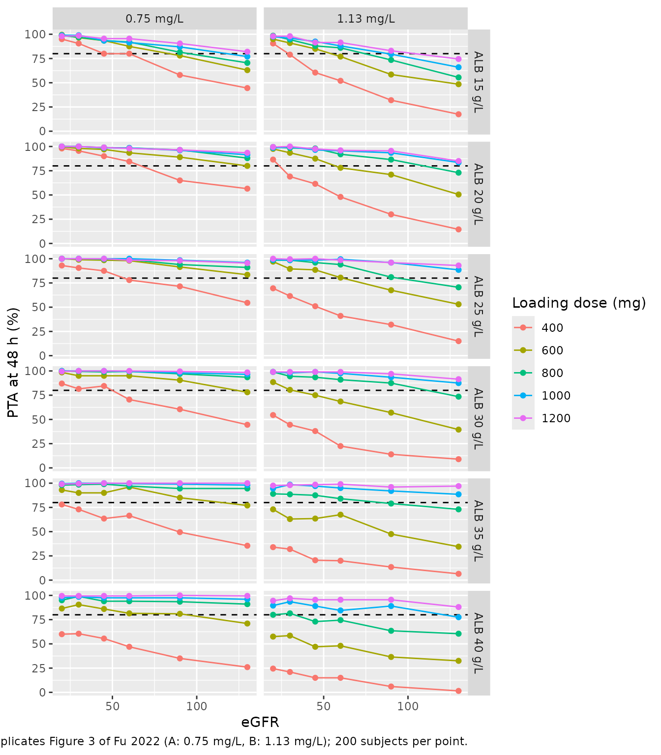
The simulated curves reproduce the figure’s pattern: PTA falls as eGFR and albumin rise, and 400 mg reaches 80% only at low eGFR or albumin. At albumin 15 g/L and eGFR 130, the 1.13 mg/L panel here puts 1200 mg at 74%, below the published point just above 80% (see the deviations below).
Assumptions and deviations
-
IIV scale. The Table 2 percentages are read as
omega x 100(variance = square). The paper does not define them; the choice follows from its own PTA table (section “IIV scale” above). -
eGFR units. The paper labels eGFR “ml/min”, but its
CKD-EPI equations (Methods Eqs 1-4) are the BSA-normalised 2009
creatinine equations and no de-normalisation is described, so the
covariate is supplied on the mL/min/1.73 m^2 scale of the canonical
CRCLcolumn. A user should compute CKD-EPI from serum creatinine (mg/dL), age and sex as printed. - Reference covariate values. Eqs 10-11 normalise by 84 (eGFR) and 32 g/L (albumin); Methods Eq 7 defines the normaliser as the covariate median. Table 1 gives only means (80.8 and 31.0).
-
Residual error. Methods Eq 6,
Y = F (1 + eps1) + eps2, is encoded as combined additive + proportional with SDs 0.122 mg/L and 0.183, taking the Table 2 eps values as standard deviations (the additive one carries concentration units). - Virtual cohort. eGFR and albumin are drawn independently from truncated normals with the Table 1 means and SDs; the paper reports no correlation.
- PTA without residual error. The PTA re-simulations use between-subject variability only; adding the residual error lowers PTA by about 3-4 points across the grid and fits Supplementary Table 1 less well.
- Extreme corner of the grid. At albumin 15 g/L (below the observed minimum of 18.3 g/L) with eGFR 90-130, the paper’s PTAs run about 5-17 points above the packaged model (for example 80.8% published versus 68.0% simulated here for 1200 mg at eGFR 130, target 1.13 mg/L; about 71% at 1000 subjects per cell). These cells have the shortest unbound half-life (about 12 h), where the trough is most sensitive to the IIV tails. The remaining cells agree within Monte Carlo error. The difference is reported, not tuned.
- Supplementary Table 1 inconsistency. The eGFR 90 / albumin 20 g/L endocarditis maintenance regimen (800/800 mg) is listed with PTA 72.6%, below the 80% criterion that defines the table (Table 3 lists the same regimen as recommended). The model agrees with the printed PTA (73.0% here, about 77% at 1000 subjects per cell), so the inconsistency is in the regimen chosen for that cell, not in the simulation. The printed value is kept as published.
- Teicoplanin product. Two products (Sanofi-Aventis and HISUN) were used; product type was screened and not retained, so the model applies to both.