Dapagliflozin, empagliflozin and canagliflozin renal SGLT1/2 QSP (Sokolov 2020)
Source:vignettes/articles/Sokolov_2020_sglt_qsp.Rmd
Sokolov_2020_sglt_qsp.RmdModel and source
- Citation: Sokolov V, Yakovleva T, Chu L, Tang W, Greasley PJ, Johansson S, Peskov K, Helmlinger G, Boulton DW, Penland RC. Differentiating the sodium-glucose cotransporter 1 inhibition capacity of canagliflozin vs. dapagliflozin and empagliflozin using quantitative systems pharmacology modeling. CPT Pharmacometrics Syst Pharmacol. 2020;9(4):222-229. doi:10.1002/psp4.12498. Model structure and parameter estimation first reported in Yakovleva T et al. Diabetes Obes Metab. 2019;21(12):2684-2693 (doi:10.1111/dom.13858); all values here are taken from the Sokolov 2020 deposited model code (Supplementary SGLT_model_code.txt).
- Description: QSP. Renal glucose filtration, SGLT2 / SGLT1-mediated reabsorption and urinary excretion in adults (healthy and type 2 diabetes mellitus) driven by the physiologically based PK of three SGLT2 inhibitors: dapagliflozin, empagliflozin and canagliflozin. Each gliflozin has an oral transit-chain absorption into a shared plasma volume (dapagliflozin with one peripheral compartment), non-renal plasma clearance, and glomerular filtration of the unbound fraction into the S1/S2 (proximal convoluted, SGLT2) and then S3 (proximal straight, SGLT1) tubular lumen, the bladder and the urine. Glucose is filtered at GFR x mean daily plasma glucose and reabsorbed by Michaelis-Menten SGLT2 (S1/S2) and SGLT1 (S3) kinetics under competitive inhibition by the luminal free drug, with disease-specific Vmax and a T2DM factor on every Ki. Mean daily plasma glucose, eGFR and T2DM status enter as covariates. Typical-value model (fit to study-level mean data); no IIV and no residual error. 37 ODE states.
- Article: https://doi.org/10.1002/psp4.12498
Sokolov et al. (2020) used a quantitative systems pharmacology (QSP)
model of renal glucose filtration, SGLT-mediated reabsorption and
urinary excretion, first reported by Yakovleva et al. (2019), to compare
how strongly dapagliflozin, empagliflozin and canagliflozin inhibit
SGLT2 (S1/S2 segments of the proximal tubule) and SGLT1 (S3 segment) in
type 2 diabetes mellitus (T2DM). The supplement deposits the complete
IQRtools model code (SGLT_model_code.txt) and the fitting /
simulation script (Script_Fitting_Simulation.R); the
packaged model is a line-by-line translation of that code.
Each gliflozin is dosed orally in mg into its own
depot_<drug> state and passes through a transit chain
into a plasma compartment of volume 2.75 L shared by all three drugs
(dapagliflozin also has a peripheral compartment). The unbound drug is
filtered at the glomerular filtration rate into the S1/S2 lumen
(pct_<drug>), flows on to the S3 lumen
(pst_<drug>), the bladder and the urine. Glucose is
filtered at GFR x GLU and reabsorbed by Michaelis-Menten
SGLT2 kinetics in S1/S2 and SGLT1 kinetics in S3. The drug free in the
tubular lumen inhibits each transporter competitively. The model is a
typical-value model fit to study-level mean data. It has no
between-subject variability and no residual error.
mod <- rxode2::rxode2(readModelDb("Sokolov_2020_sglt_qsp"))
mw <- c(dapagliflozin = 408.87, empagliflozin = 450.91, canagliflozin = 444.5)
drugs <- names(mw)
drug_cols <- c(dapagliflozin = "#E41A1C", empagliflozin = "#377EB8", canagliflozin = "#4DAF4A")
Population
The model was fit to published, study-level mean data from phase I and II trials in healthy volunteers and adults with T2DM (Sokolov 2020 Table S1): plasma concentration-time profiles, 24-hour urinary drug excretion and 24-hour urinary glucose excretion (UGE). Each trial arm’s mean daily plasma glucose (MPG) and eGFR were supplied as regressors. The pharmacodynamic T2DM data set comprised 7 dapagliflozin arms (2.5-100 mg), 11 canagliflozin arms (25-400 mg) and 14 empagliflozin arms (1-100 mg). Median MPG was 7.8, 9.24 and 10.43 mM, and median eGFR 98.1, 100 and 100 mL/min/1.73 m^2, in the dapagliflozin, empagliflozin and canagliflozin trials respectively; the pooled T2DM medians were 9.33 mM and 100 mL/min/1.73 m^2 (Table S2). Subject counts and demographics are not reported because only arm means were modelled.
The same information is available programmatically via
readModelDb("Sokolov_2020_sglt_qsp")()$population.
Source trace
Every ini() value comes from the
MODEL PARAMETERS section of the deposited
SGLT_model_code.txt and carries an in-file comment. The
ODEs and rate laws are Sokolov 2020 Table S3. Where Table S3 and the
code differ, the code is followed; see Assumptions and
deviations.
| Equation / parameter | Value | Source location |
|---|---|---|
lvc (plasma volume, all drugs) |
log(2.75 L), fixed | Code Vpl
|
v_pct, v_pst, v_bladder
|
0.045, 0.01944, 0.2 L, fixed | Code Vlumen1, Vlumen2,
Vbladder
|
q_pct, q_pst, q_urine
|
2.7, 0.72, 0.055 L/h, fixed | Code Qlumen, Qbladder,
Qurine
|
lfdepot_* |
0.78 / 0.78 / 0.65, fixed | Code Fdapa, Fempa, Fcana
|
fu_* |
0.086 / 0.22 / 0.01, fixed | Code fupdapa, fupempa,
fupcana
|
mw_*, mw_glucose
|
408.87 / 450.91 / 444.5 / 180.156 g/mol, fixed | Code MW*
|
lktr_* |
10.38 / 19.8 / 11.93 1/h | Code k_tr_d, k_tr_e,
k_tr_c
|
lka_* |
0.5071 / 0.09984 / 0.1358 1/h | Code kabs*
|
lcl_* |
13.07 / 5.78 / 8.242 L/h | Code CL*pls
|
lq_dapagliflozin, lvp_dapagliflozin
|
13.65 L/h, 98.57 L | Code Qdapa, Vprfdapa
|
km_sglt2, km_sglt1
|
4, 0.5 mM, fixed | Code KmreabsSGLT2, KmreabsSGLT1
|
vmax_total_healthy, vmax_total_t2dm
|
105.6, 140 mmol/h, fixed | Code Vmax_hs, Vmax_t2d
|
lvmax_sglt2_healthy, lvmax_sglt2_t2dm
|
87.07, 111.4 mmol/h | Code VmaxreabsSGLT2hs,
VmaxreabsSGLT2t2d
|
lki_sglt2_* (healthy) |
103.1 / 638.6 / 364.3 pM | Code Ki*SGLT2ex
|
ratio_sglt1_* |
1157 / 1249 / 158, fixed | Code Ki*SGLT1ex expressions (in vitro SGLT1:SGLT2
ratio) |
f_ki_t2dm |
0.3047 | Code coef
|
reabs_base |
39.174 mmol/h, fixed | Code reabsbase
|
| Transit chains (5 / 5 / 4 states) | n/a | Code MODEL REACTIONS Vtr*_d,
Vtr*_e, Vtr*_c
|
| Drug disposition ODEs | n/a | Table S3 (Dapagliflozin / Empagliflozin / Canagliflozin blocks) |
| SGLT2 / SGLT1 reabsorption rate laws | n/a | Table S3 V_reabs1, V_reabs2; code
reabsSGLT2dr, reabsSGLT1dr
|
| T2DM Ki factor and Vmax switch | n/a | Code khs / kt2d terms in
reabsSGLT*dr
|
GFR from eGFR (CRCL * 60 / 1000) |
n/a | Script, Figure 1 block (GFR * 1000 / 60) |
The six SGLT parameters (lvmax_sglt2_*,
lki_sglt2_*, f_ki_t2dm) are the ones the
deposited script estimates; the PK parameters were estimated in the
companion analysis. Together these are the paper’s 17 estimated
parameters. The 27 literature parameters are fixed().
Exact gates on derived quantities
The T2DM Ki values in Table 1 are not model parameters. They are
derived from the healthy SGLT2 Ki, the T2DM factor and the in vitro
ratio. The glucose filtration fluxes in Table S2 are
GFR x MPG. Both must reproduce exactly.
ini_df <- mod$iniDf
th <- setNames(ini_df$est, ini_df$name)
ki2_t2dm <- exp(th[paste0("lki_sglt2_", drugs)]) * th[["f_ki_t2dm"]] / 1000 # nM
ki1_t2dm <- ki2_t2dm * th[paste0("ratio_sglt1_", drugs)]
ki_tbl <- data.frame(
  drug = drugs,
  ki2_model = unname(ki2_t2dm), ki2_table1 = c(0.031, 0.195, 0.111),
  ki1_model = unname(ki1_t2dm), ki1_table1 = c(36.35, 243.03, 17.55)
)
knitr::kable(
  ki_tbl |>
    dplyr::rename(
      "Drug" = drug,
      "Ki SGLT2 model (nM)" = ki2_model, "Ki SGLT2 Table 1 (nM)" = ki2_table1,
      "Ki SGLT1 model (nM)" = ki1_model, "Ki SGLT1 Table 1 (nM)" = ki1_table1
    ),
  digits = 3,
  caption = "T2DM inhibitory constants derived from the packaged parameters versus Sokolov 2020 Table 1."
)| Drug | Ki SGLT2 model (nM) | Ki SGLT2 Table 1 (nM) | Ki SGLT1 model (nM) | Ki SGLT1 Table 1 (nM) |
|---|---|---|---|---|
| dapagliflozin | 0.031 | 0.031 | 36.347 | 36.35 |
| empagliflozin | 0.195 | 0.195 | 243.032 | 243.03 |
| canagliflozin | 0.111 | 0.111 | 17.538 | 17.55 |
# Table 1 prints the SGLT2 Ki to 3 decimals. The SGLT1 Ki agree to 0.1%: the
# canagliflozin value is 17.538 nM here and in the deposited script's own
# Figure 4 block (57.559 * 0.3047), against 17.55 printed in Table 1.
stopifnot(
  all(abs(ki_tbl$ki2_model - ki_tbl$ki2_table1) <= 0.0005 + 1e-9),
  all(abs(ki_tbl$ki1_model / ki_tbl$ki1_table1 - 1) < 1e-3)
)

flux <- data.frame(
  scenario = c("dapagliflozin", "empagliflozin", "canagliflozin", "common"),
  mpg = c(7.8, 9.24, 10.43, 9.33),
  egfr = c(98.1, 100, 100, 100),
  flux_tableS2 = c(45.89, 55.48, 62.61, 55.98)
) |>
  dplyr::mutate(flux_model = egfr * 60 / 1000 * mpg)
# Table S2 prints the medians rounded (e.g. MPG 7.8 mM) while its flux column
# is the product of the unrounded medians, so agreement is to 0.1%, not exact.
stopifnot(all(abs(flux$flux_model / flux$flux_tableS2 - 1) < 2e-3))
Steady-state initial condition
The deposited code starts the tubular glucose states at zero and runs a 72-h drug-free burn-in before dosing. The packaged model instead starts each glucose state at its drug-free steady state, so a dose can be given at time 0. Without a dose, the glucose states and the UGE rate must stay constant over the whole simulation.
make_subject <- function(id, drug, dose, glu = 9.33, egfr = 100, t2dm = 1,
                         times = seq(0, 24, by = 0.1)) {
  dose_row <- data.frame(
    id = id, time = 0, evid = 1, amt = dose, cmt = paste0("depot_", drug)
  )
  obs_rows <- data.frame(
    id = id, time = times, evid = 0, amt = 0, cmt = paste0("central_", drug)
  )
  dplyr::bind_rows(dose_row, obs_rows) |>
    dplyr::mutate(GLU = glu, CRCL = egfr, DIS_DIAB = t2dm, drug = drug, dose = dose)
}
solve_df <- function(d, m = mod) {
  as.data.frame(rxode2::rxSolve(m, d, keep = c("drug", "dose"), returnType = "data.frame"))
}

pbo <- solve_df(make_subject(1, "dapagliflozin", 0, times = seq(0, 200, by = 1)))
drift <- pbo |>
  dplyr::summarise(
    dplyr::across(c(glu_pct, glu_pst, glu_bladder), ~ max(abs(.x / .x[1] - 1)))
  )
uge_rate <- diff(pbo$uge) / diff(pbo$time)
stopifnot(
  all(unlist(drift) < 1e-6),
  max(abs(uge_rate / uge_rate[1] - 1)) < 1e-6
)
drift
#>        glu_pct      glu_pst  glu_bladder
#> 1 4.440892e-16 6.661338e-15 6.328271e-15
Table 1: drug concentrations in plasma, kidney and bladder
Single oral doses at the highest approved doses (dapagliflozin 10 mg, empagliflozin 25 mg, canagliflozin 300 mg) in a typical T2DM subject with the common median MPG (9.33 mM) and eGFR (100 mL/min/1.73 m^2). As in the deposited script, the 0-24 h average is the mean over a 0.1-h output grid.
approved <- c(dapagliflozin = 10, empagliflozin = 25, canagliflozin = 300)
typ <- dplyr::bind_rows(lapply(seq_along(drugs), function(i) {
  make_subject(i, drugs[i], approved[[drugs[i]]], times = seq(0, 120, by = 0.1))
})) |>
  solve_df()

conc_long <- dplyr::bind_rows(lapply(drugs, function(d) {
  s <- typ[typ$drug == d, ]
  data.frame(
    drug = d, time = s$time,
    Plasma = s[[paste0("Cc_", d)]] / mw[[d]] * 1000,
    `S1-S2` = s[[paste0("pct_", d)]] / 0.045 * 1e6,
    S3 = s[[paste0("pst_", d)]] / 0.01944 * 1e6,
    Bladder = s[[paste0("bladder_", d)]] / 0.2 * 1e6,
    check.names = FALSE
  )
})) |>
  tidyr::pivot_longer(c(Plasma, `S1-S2`, S3, Bladder), names_to = "site", values_to = "conc_nM")

t1_sim <- conc_long |>
  dplyr::filter(time <= 24) |>
  dplyr::group_by(drug, site) |>
  dplyr::summarise(cmax = max(conc_nM), cavg = mean(conc_nM), .groups = "drop")

t1_ref <- data.frame(
  drug = rep(drugs, each = 4),
  site = rep(c("Plasma", "S1-S2", "S3", "Bladder"), 3),
  cmax_ref = c(275, 52.5, 196, 987, 533, 260, 976, 8172, 6156, 137, 513, 3922),
  cavg_ref = c(51.7, 9.87, 37.0, 462, 229, 112, 420, 5164, 2109, 46.9, 176, 2205)
)
t1 <- dplyr::left_join(t1_ref, t1_sim, by = c("drug", "site")) |>
  dplyr::mutate(
    cmax_pct = 100 * (cmax - cmax_ref) / cmax_ref,
    cavg_pct = 100 * (cavg - cavg_ref) / cavg_ref
  )
knitr::kable(
  t1 |>
    dplyr::select(drug, site, cmax_ref, cmax, cmax_pct, cavg_ref, cavg, cavg_pct) |>
    dplyr::rename(
      "Drug" = drug, "Site" = site,
      "Cmax Table 1 (nM)" = cmax_ref, "Cmax model (nM)" = cmax, "Cmax % diff" = cmax_pct,
      "Cavg0-24 Table 1 (nM)" = cavg_ref, "Cavg0-24 model (nM)" = cavg, "Cavg % diff" = cavg_pct
    ),
  digits = 2,
  caption = "Replicates Table 1 of Sokolov 2020 (model-predicted Cmax and Cavg0-24)."
)| Drug | Site | Cmax Table 1 (nM) | Cmax model (nM) | Cmax % diff | Cavg0-24 Table 1 (nM) | Cavg0-24 model (nM) | Cavg % diff |
|---|---|---|---|---|---|---|---|
| dapagliflozin | Plasma | 275.0 | 274.98 | -0.01 | 51.70 | 51.46 | -0.46 |
| dapagliflozin | S1-S2 | 52.5 | 52.51 | 0.03 | 9.87 | 9.83 | -0.37 |
| dapagliflozin | S3 | 196.0 | 196.30 | 0.16 | 37.00 | 36.87 | -0.36 |
| dapagliflozin | Bladder | 987.0 | 986.79 | -0.02 | 462.00 | 460.75 | -0.27 |
| empagliflozin | Plasma | 533.0 | 532.55 | -0.08 | 229.00 | 228.30 | -0.30 |
| empagliflozin | S1-S2 | 260.0 | 260.36 | 0.14 | 112.00 | 111.60 | -0.36 |
| empagliflozin | S3 | 976.0 | 976.16 | 0.02 | 420.00 | 418.36 | -0.39 |
| empagliflozin | Bladder | 8172.0 | 8171.78 | 0.00 | 5164.00 | 5146.70 | -0.34 |
| canagliflozin | Plasma | 6156.0 | 6155.80 | 0.00 | 2109.00 | 2100.90 | -0.38 |
| canagliflozin | S1-S2 | 137.0 | 136.81 | -0.14 | 46.90 | 46.68 | -0.46 |
| canagliflozin | S3 | 513.0 | 512.99 | 0.00 | 176.00 | 175.03 | -0.55 |
| canagliflozin | Bladder | 3922.0 | 3921.94 | 0.00 | 2205.00 | 2196.94 | -0.37 |
# Same parameters and same deterministic model as the paper's simulation; the
# residual difference is rounding of the printed values and the output grid.
stopifnot(
  nrow(t1) == 12L, !anyNA(t1$cmax), !anyNA(t1$cavg),
  max(abs(t1$cmax_pct)) < 1,
  max(abs(t1$cavg_pct)) < 2
)
ggplot(conc_long |> dplyr::filter(time <= 120), aes(time / 24, conc_nM, colour = drug)) +
  geom_line(linewidth = 0.8) +
  facet_wrap(~site, nrow = 1) +
  scale_y_log10(limits = c(1e-5, 1e4)) +
  scale_colour_manual(values = drug_cols) +
  labs(x = "Time (days)", y = "Free drug concentration (nM)", colour = NULL) +
  theme_bw() +
  theme(legend.position = "bottom")
#> Warning in scale_y_log10(limits = c(1e-05, 10000)): log-10 transformation
#> introduced infinite values.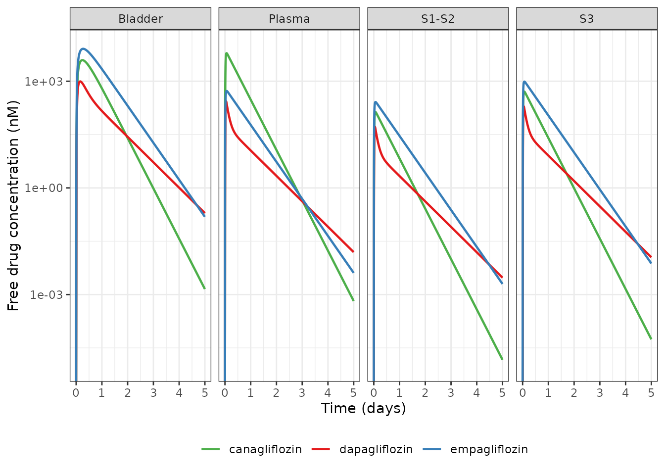
Replicates Figure 3 (top row) of Sokolov 2020: drug concentrations in plasma, the S1/S2 and S3 tubular lumen and the bladder after a single approved dose.
Figure 3 (bottom row): reabsorption and cumulative UGE
pbo5 <- solve_df(make_subject(99, "dapagliflozin", 0, times = seq(0, 120, by = 0.1)))
reabs <- typ |>
  dplyr::left_join(pbo5 |> dplyr::select(time, uge_pbo = uge), by = "time") |>
  dplyr::group_by(drug) |>
  dplyr::mutate(
    `Total reabsorption (% of max)` = 100 * reabs_total / max(reabs_total),
    `SGLT1 contribution (%)` = 100 * reabs_sglt1 / reabs_total,
    `SGLT2 contribution (%)` = 100 * reabs_sglt2 / reabs_total,
    `Placebo-normalized cumulative UGE (g)` = uge - uge_pbo
  ) |>
  dplyr::ungroup()
reabs |>
  dplyr::select(drug, time, dplyr::ends_with("(%)"), dplyr::ends_with("of max)"), dplyr::ends_with("(g)")) |>
  tidyr::pivot_longer(-c(drug, time)) |>
  ggplot(aes(time / 24, value, colour = drug)) +
  geom_line(linewidth = 0.8) +
  facet_wrap(~name, nrow = 1, scales = "free_y") +
  scale_colour_manual(values = drug_cols) +
  labs(x = "Time (days)", y = NULL, colour = NULL) +
  theme_bw() +
  theme(legend.position = "bottom")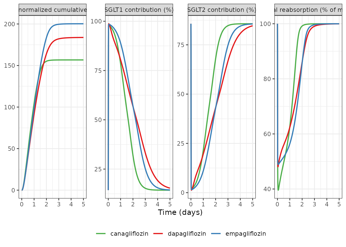
The Results report a 24-hour UGE of 92 g (dapagliflozin), 98 g (empagliflozin) and 104 g (canagliflozin), and a placebo-normalized cumulative UGE over 0-5 days of 184, 200 and 157 g.
uge_tbl <- reabs |>
  dplyr::group_by(drug) |>
  dplyr::summarise(
    uge24 = uge[time == 24],
    uge_cum5 = `Placebo-normalized cumulative UGE (g)`[time == 120]
  ) |>
  dplyr::left_join(
    data.frame(drug = drugs, uge24_ref = c(92, 98, 104), uge_cum5_ref = c(184, 200, 157)),
    by = "drug"
  )
knitr::kable(
  uge_tbl |>
    dplyr::select(drug, uge24_ref, uge24, uge_cum5_ref, uge_cum5) |>
    dplyr::rename(
      "Drug" = drug, "24-h UGE paper (g)" = uge24_ref, "24-h UGE model (g)" = uge24,
      "0-5 d placebo-normalized UGE paper (g)" = uge_cum5_ref,
      "0-5 d placebo-normalized UGE model (g)" = uge_cum5
    ),
  digits = 1,
  caption = "24-hour and cumulative UGE after a single approved dose (Sokolov 2020 Results)."
)| Drug | 24-h UGE paper (g) | 24-h UGE model (g) | 0-5 d placebo-normalized UGE paper (g) | 0-5 d placebo-normalized UGE model (g) |
|---|---|---|---|---|
| canagliflozin | 104 | 104.9 | 157 | 156.7 |
| dapagliflozin | 92 | 92.0 | 184 | 183.8 |
| empagliflozin | 98 | 99.0 | 200 | 200.3 |
Figure 2: UGE dose response in T2DM
The deposited script simulates the 24-h UGE after a single dose. It does this under two scenarios: the “in situ” scenario uses drug-specific median MPG and eGFR (Figure 2a), and the “normalized” scenario uses the common medians (Figure 2b).
doses <- c(0.1, 0.25, 0.5, 1, 2.5, 5, 10, 25, 50, 100, 300, 1000)
scen <- data.frame(
  scenario = c(rep("in situ", 3), rep("normalized", 3)),
  drug = rep(drugs, 2),
  glu = c(7.8, 9.24, 10.43, rep(9.33, 3)),
  egfr = c(98.1, 100, 100, rep(100, 3))
)
dr_events <- list()
id <- 0L
for (k in seq_len(nrow(scen))) {
  for (dz in doses) {
    id <- id + 1L
    dr_events[[id]] <- make_subject(id, scen$drug[k], dz,
      glu = scen$glu[k], egfr = scen$egfr[k], times = 24
    ) |>
      dplyr::mutate(scenario = scen$scenario[k])
  }
}
dr_events <- dplyr::bind_rows(dr_events)
dr <- as.data.frame(rxode2::rxSolve(mod, dr_events,
  keep = c("drug", "dose", "scenario"), returnType = "data.frame"
))

ggplot(dr, aes(dose, uge, colour = drug)) +
  geom_line(linewidth = 0.8) +
  geom_point() +
  facet_wrap(~scenario) +
  scale_x_log10() +
  scale_colour_manual(values = drug_cols) +
  coord_cartesian(ylim = c(0, 180)) +
  labs(x = "Dose (mg)", y = "24-h UGE (g/day)", colour = NULL) +
  theme_bw() +
  theme(legend.position = "bottom")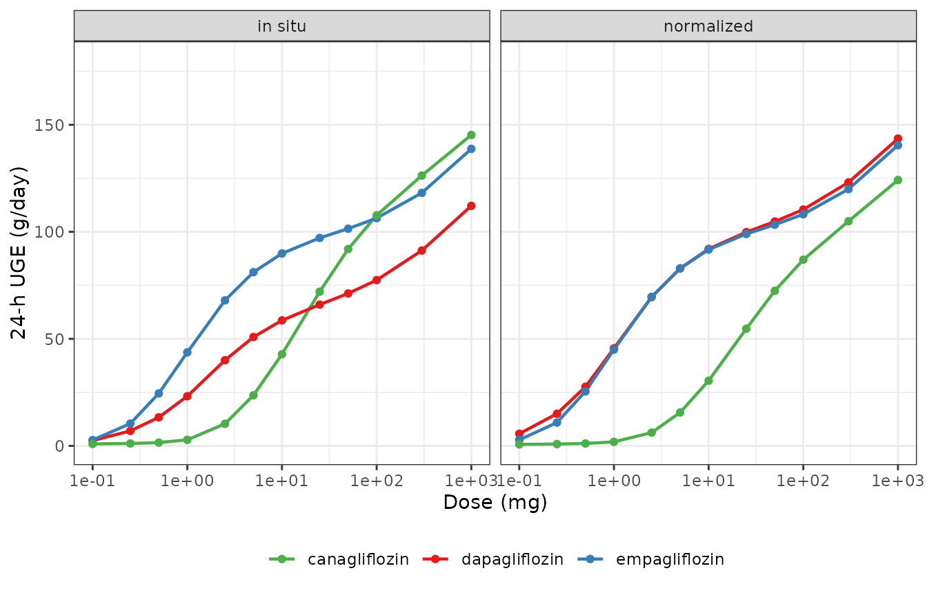
Replicates Figure 2 of Sokolov 2020 (model curves only; the observed arm means are in the unpublished analysis data set).
In the normalized scenario the Results state that the UGE is 82.3 and 91.4 g/day for 5 and 10 mg dapagliflozin, 91.1 and 98.4 g/day for 10 and 25 mg empagliflozin, and 86.4 and 104.3 g for 100 and 300 mg canagliflozin.
uge24_pbo <- pbo$uge[pbo$time == 24]
dr_ref <- data.frame(
  drug = rep(drugs, each = 2),
  dose = c(5, 10, 10, 25, 100, 300),
  uge_ref = c(82.3, 91.4, 91.1, 98.4, 86.4, 104.3)
)
dr_cmp <- dr |>
  dplyr::filter(scenario == "normalized") |>
  dplyr::select(drug, dose, uge) |>
  dplyr::inner_join(dr_ref, by = c("drug", "dose")) |>
  dplyr::mutate(
    pct = 100 * (uge - uge_ref) / uge_ref,
    uge_net = uge - uge24_pbo,
    pct_net = 100 * (uge_net - uge_ref) / uge_ref
  )
knitr::kable(
  dr_cmp |>
    dplyr::select(drug, dose, uge_ref, uge, pct, uge_net, pct_net) |>
    dplyr::rename(
      "Drug" = drug, "Dose (mg)" = dose, "UGE paper (g/day)" = uge_ref,
      "Total UGE model (g/day)" = uge, "% diff (total)" = pct,
      "UGE minus drug-free baseline (g/day)" = uge_net, "% diff (net)" = pct_net
    ),
  digits = 2,
  caption = "Normalized-scenario 24-h UGE (Sokolov 2020 Results, Figure 2b)."
)| Drug | Dose (mg) | UGE paper (g/day) | Total UGE model (g/day) | % diff (total) | UGE minus drug-free baseline (g/day) | % diff (net) |
|---|---|---|---|---|---|---|
| dapagliflozin | 5 | 82.3 | 82.91 | 0.74 | 82.31 | 0.01 |
| dapagliflozin | 10 | 91.4 | 92.00 | 0.65 | 91.39 | -0.01 |
| empagliflozin | 10 | 91.1 | 91.70 | 0.66 | 91.10 | 0.00 |
| empagliflozin | 25 | 98.4 | 98.98 | 0.59 | 98.38 | -0.02 |
| canagliflozin | 100 | 86.4 | 86.99 | 0.68 | 86.38 | -0.02 |
| canagliflozin | 300 | 104.3 | 104.93 | 0.60 | 104.32 | 0.02 |
The total 24-h UGE is 0.6-0.7% above every value in the Results paragraph. The offset equals the drug-free 24-h UGE (0.6 g). With that baseline subtracted, all six values agree to within 0.1%. The paragraph therefore appears to report UGE net of the drug-free baseline, although the paper does not say so. The separate statement that the 24-h UGE after the approved doses is 92, 98 and 104 g matches the total UGE (previous section).
Figure 4: SGLT1 exposure and contribution to UGE
Figure 4a compares the average S3 concentration over the 24 h after
dosing with the T2DM SGLT1 Ki. Figure 4b gives the share of 24-h UGE
that is due to SGLT1 inhibition. The script computes it by re-running
the model with SGLT1 inhibition switched off (the code’s
k_sglt1 = 1e8, which multiplies every SGLT1 Ki), and the
packaged model does the same through the ratio_sglt1_*
parameters. The paper reports S3 exposure ratios of 0.5 (dapagliflozin 5
mg), 1.0 (dapagliflozin 10 mg), 1.7 (empagliflozin 25 mg) and 10
(canagliflozin 300 mg), and SGLT1 contributions of 1.59%, 2.41% and
about 10%.
mod_no_sglt1 <- rxode2::ini(
  mod,
  ratio_sglt1_dapagliflozin = fixed(1157e8),
  ratio_sglt1_empagliflozin = fixed(1249e8),
  ratio_sglt1_canagliflozin = fixed(158e8)
)
#> Warning: trying to fix 'ratio_sglt1_dapagliflozin', but already fixed
#> ℹ change initial estimate of `ratio_sglt1_dapagliflozin` to `1.157e+11`
#> Warning: trying to fix 'ratio_sglt1_empagliflozin', but already fixed
#> ℹ change initial estimate of `ratio_sglt1_empagliflozin` to `1.249e+11`
#> Warning: trying to fix 'ratio_sglt1_canagliflozin', but already fixed
#> ℹ change initial estimate of `ratio_sglt1_canagliflozin` to `1.58e+10`
f4_events <- dplyr::bind_rows(
  make_subject(1, "dapagliflozin", 5),
  make_subject(2, "dapagliflozin", 10),
  make_subject(3, "empagliflozin", 25),
  make_subject(4, "canagliflozin", 300)
)
f4_on <- solve_df(f4_events)
f4_off <- solve_df(f4_events, mod_no_sglt1)
ki1_named <- setNames(ki1_t2dm, drugs)
f4 <- f4_on |>
  dplyr::group_by(id, drug, dose) |>
  dplyr::summarise(
    cavg_s3 = mean(dplyr::case_when(
      drug == "dapagliflozin" ~ pst_dapagliflozin,
      drug == "empagliflozin" ~ pst_empagliflozin,
      TRUE ~ pst_canagliflozin
    ) / 0.01944 * 1e6),
    uge_on = uge[time == 24],
    .groups = "drop"
  ) |>
  dplyr::left_join(
    f4_off |> dplyr::filter(time == 24) |> dplyr::select(id, uge_off = uge),
    by = "id"
  ) |>
  dplyr::mutate(
    ratio_s3 = cavg_s3 / ki1_named[drug],
    sglt1_share = 100 * (uge_on - uge_off) / uge_on,
    ratio_ref = c(0.5, 1.0, 1.7, 10),
    share_ref = c(NA, 1.59, 2.41, 10)
  )
knitr::kable(
  f4 |>
    dplyr::select(drug, dose, ratio_ref, ratio_s3, share_ref, sglt1_share) |>
    dplyr::rename(
      "Drug" = drug, "Dose (mg)" = dose,
      "Cavg S3 / Ki SGLT1 paper" = ratio_ref, "Cavg S3 / Ki SGLT1 model" = ratio_s3,
      "SGLT1 share of UGE paper (%)" = share_ref, "SGLT1 share of UGE model (%)" = sglt1_share
    ),
  digits = 2,
  caption = "Replicates Figure 4 of Sokolov 2020."
)| Drug | Dose (mg) | Cavg S3 / Ki SGLT1 paper | Cavg S3 / Ki SGLT1 model | SGLT1 share of UGE paper (%) | SGLT1 share of UGE model (%) |
|---|---|---|---|---|---|
| dapagliflozin | 5 | 0.5 | 0.51 | NA | 0.98 |
| dapagliflozin | 10 | 1.0 | 1.01 | 1.59 | 1.62 |
| empagliflozin | 25 | 1.7 | 1.72 | 2.41 | 2.45 |
| canagliflozin | 300 | 10.0 | 9.98 | 10.00 | 10.81 |
stopifnot(
  # Exposure ratios are printed to 1-2 significant figures.
  all(abs(f4$ratio_s3 - f4$ratio_ref) / f4$ratio_ref < 0.06),
  # The two exact SGLT1 shares; the canagliflozin value is printed as ~10 %.
  all(abs(f4$sglt1_share[2:3] - f4$share_ref[2:3]) < 0.1),
  abs(f4$sglt1_share[4] - 10) < 1
)

ggplot(f4 |> dplyr::filter(dose != 5), aes(drug, sglt1_share, fill = drug)) +
  geom_col(colour = "black", show.legend = FALSE) +
  geom_text(aes(label = sprintf("%.2f%%", sglt1_share)), vjust = -0.5) +
  scale_fill_manual(values = drug_cols) +
  labs(x = NULL, y = "SGLT1 contribution to 24-h UGE (%)") +
  theme_bw()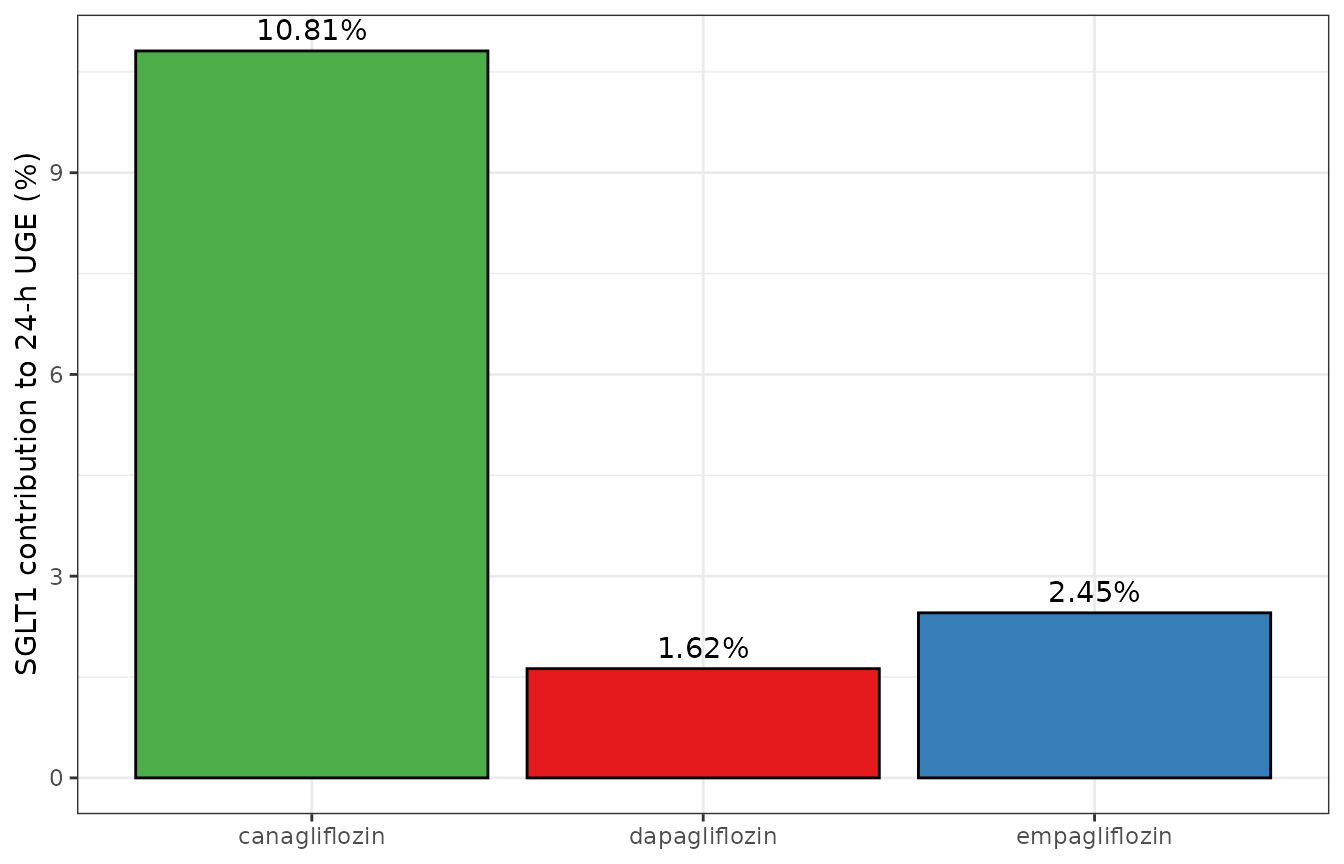
The S3 exposure ratios reproduce Figure 4a. The SGLT1 shares of 24-h UGE are 1.62% and 2.45% for dapagliflozin and empagliflozin, against 1.59% and 2.41% printed. They are small differences between two nearly equal UGE values (about 0.03 g of about 92 g), which the rounding of the deposited parameter values can explain. Canagliflozin gives 10.8%, against “approximately 10%” in the text and a bar labelled 10 in Figure 4b.
PKNCA: plasma exposure after a single approved dose
nca_conc <- conc_long |>
  dplyr::filter(site == "Plasma", time <= 24) |>
  dplyr::mutate(id = match(drug, drugs), treatment = drug) |>
  dplyr::filter(!is.na(conc_nM))
nca_dose <- data.frame(
  id = seq_along(drugs), time = 0, treatment = drugs,
  dose_nmol = unname(approved[drugs] / mw[drugs] * 1e6)
)
conc_obj <- PKNCA::PKNCAconc(nca_conc, conc_nM ~ time | treatment + id)
dose_obj <- PKNCA::PKNCAdose(nca_dose, dose_nmol ~ time | treatment + id)
intervals <- data.frame(start = 0, end = 24, cmax = TRUE, tmax = TRUE, auclast = TRUE, cav = TRUE)
nca_res <- PKNCA::pk.nca(PKNCA::PKNCAdata(conc_obj, dose_obj, intervals = intervals))

nca_ref <- data.frame(
  treatment = drugs,
  cmax = c(275, 533, 6156),
  cav = c(51.7, 229, 2109)
)
cmp <- nlmixr2lib::ncaComparisonTable(
  simulated = nca_res,
  reference = nca_ref,
  by = "treatment",
  units = c(cmax = "nM", cav = "nM"),
  tolerance_pct = 20
)
knitr::kable(
  cmp,
  caption = paste(
    "PKNCA plasma Cmax and 0-24 h average concentration after a single",
    "approved dose versus Sokolov 2020 Table 1 (plasma rows).",
    "* marks a difference above 20%."
  )
)| NCA parameter | treatment | Reference | Simulated | % diff |
|---|---|---|---|---|
| Cmax (nM) | dapagliflozin | 275 | 275 | -0.0% |
| Cmax (nM) | empagliflozin | 533 | 533 | -0.1% |
| Cmax (nM) | canagliflozin | 6160 | 6160 | -0.0% |
| Cavg (nM) | dapagliflozin | 51.7 | 51.7 | -0.1% |
| Cavg (nM) | empagliflozin | 229 | 229 | +0.1% |
| Cavg (nM) | canagliflozin | 2110 | 2110 | +0.0% |
nca_num <- as.data.frame(nca_res$result) |>
  dplyr::filter(PPTESTCD %in% c("cmax", "cav")) |>
  dplyr::select(treatment, PPTESTCD, sim = PPORRES) |>
  dplyr::left_join(
    tidyr::pivot_longer(nca_ref, -treatment, names_to = "PPTESTCD", values_to = "ref"),
    by = c("treatment", "PPTESTCD")
  )
# One deterministic typical subject per drug; the only difference from the
# paper is the linear-trapezoid AUC versus the grid mean used for Table 1.
stopifnot(nrow(nca_num) == 6L, max(abs(nca_num$sim / nca_num$ref - 1)) < 0.02)
All three drugs reproduce Table 1 closely, and no row is flagged.
Assumptions and deviations
-
Code over Table S3. The deposited code has 5
(dapagliflozin), 5 (empagliflozin) and 4 (canagliflozin) first-order
transit states between the dosing state and plasma. Table S3 writes
absorption directly from the dosing state and omits them. Table S3 also
shows no T2DM factor on Ki and prints
Cana_lumen1in the glucoseV_lumenrate law. The packaged model follows the code throughout. With the code’s structure, Table 1, the Figure 2 UGE values and the Figure 4 SGLT1 shares all reproduce (see the gates above). The T2DM Ki in Table 1 equal the healthy Ki timescoef, which confirms the factor. - Steady-state glucose start. The code starts the tubular glucose states at zero and burns in for 72 h. The packaged model starts them at the analytic drug-free steady state, so a dose can be given at time 0. The steady-state gate above confirms the two are equivalent.
-
Plasma glucose is not a state. Mean daily plasma
glucose (
GLU) is a per-subject input and is not lowered by the drug. This is the paper’s own stated limitation: it considered only 24-h mean glucose and cumulative UGE. -
eGFR used as absolute GFR. GFR in L/h is
CRCL * 60 / 1000, as in the deposited script. The BSA-normalized eGFR is not de-normalized. -
Omitted bookkeeping. The code’s AUC accumulator
states and its urine-reset events at fixed times are not carried. They
are output bookkeeping for particular simulations. AUCs and interval UGE
are computed from the output instead
(e.g.
uge(t2) - uge(t1)). The code’sk_sglt1switch is reproduced by scaling theratio_sglt1_*parameters (Figure 4 section). - No variability. The fit used mean data and the error-model estimates are not reported. The model therefore has no IIV and no residual error, and is intended for typical-value simulation.
-
Tubular fluid specimen. The tubular-lumen states
are recorded with specimen
urine(glomerular filtrate on its way to the bladder), the closest term in the controlled vocabulary.