Colistin (Karaiskos 2015)
Source:vignettes/articles/Karaiskos_2015_colistin.Rmd
Karaiskos_2015_colistin.RmdModel and source
- Citation: Karaiskos I, Friberg LE, Pontikis K, Ioannidis K, Tsagkari V, Galani L, Kostakou E, Baziaka F, Paskalis C, Koutsoukou A, Giamarellou H. Colistin population pharmacokinetics after application of a loading dose of 9 MU colistin methanesulfonate in critically ill patients. Antimicrob Agents Chemother. 2015;59(12):7240-7248.
- Article: https://doi.org/10.1128/AAC.00554-15
The model captures the slow in vivo conversion of colistimethate sodium (CMS, the inactive prodrug administered intravenously) to colistin (the active polymyxin) by a chain of hydrolysis steps through partially-sulfomethylated intermediates. Karaiskos 2015 pools the new 9 MU loading-dose cohort (19 ICU patients) with two earlier critically-ill cohorts (3 MU q8h and 6 MU loading plus 3 MU q8h) for a total of 47 patients and 1144 plasma concentrations.
Population
Nineteen critically ill adults (11 men, 8 women) admitted to two Athens hospitals received intravenous CMS for extensively drug-resistant Gram-negative infections (XDR Acinetobacter baumannii n=8, XDR Pseudomonas aeruginosa n=5, carbapenemase-producing Klebsiella pneumoniae n=3, Citrobacter sp. n=1, plus two empirical cases). Mean age was 56.2 years (range 18-86), median creatinine clearance was 92.1 mL/min on day 1 (capped at 150 mL/min in the analysis), mean APACHE II score was 18.4, and mean serum albumin was 2.8 g/dL. Karaiskos 2015 Table 1 lists baseline demographics for the new cohort; the population PK analysis pools these subjects with 28 additional patients from two prior studies cited in the paper, for a fitting dataset of 47 patients.
The dosing regimen for the new study was a 9 MU CMS loading dose (~270 mg colistin base activity; ~413 umol CMS) over either 30 or 60 minutes, followed 24 h later by 4.5 MU q12h maintenance (with dose reduction per the modified Garonzik formula for CrCL < 60 mL/min). Patients on renal replacement were excluded.
The same information is available programmatically via the model’s
population metadata
(readModelDb("Karaiskos_2015_colistin")$population).
Source trace
Per-parameter origin is recorded as an in-file comment next to each
ini() entry in
inst/modeldb/specificDrugs/Karaiskos_2015_colistin.R. The
table below collects them in one place for review.
| Equation / parameter | Value | Source location |
|---|---|---|
lcl_nonren = log(CL_NR) |
log(5.84) L/h | Karaiskos 2015 Table 2 CMS column (11% RSE) |
e_crcl_cl_renal = Sl_CRCL |
0.541 | Karaiskos 2015 Table 2 (16% RSE) |
lvc = log(V1) |
log(1.42) L | Karaiskos 2015 Table 2 CMS column (13% RSE) |
lvp = log(V2) |
log(12.5) L | Karaiskos 2015 Table 2 CMS column (10% RSE) |
lq = log(Q1) |
log(550) L/h | Karaiskos 2015 Table 2 CMS column (31% RSE) |
lq_cms2 = log(Q2) |
log(7.75) L/h | Karaiskos 2015 Table 2 CMS column (11% RSE) |
lcl_col = log(CL/fm) |
log(4.99) L/h | Karaiskos 2015 Table 2 colistin column (25% RSE) |
lvc_col = log(V/fm) |
log(80.4) L | Karaiskos 2015 Table 2 colistin column (11% RSE) |
etalcl_nonren (IIV CMS CL) |
0.02528 (16% CV) | Karaiskos 2015 Table 2 IIV column (37% RSE) |
etalcl_col (IIV col CL) |
0.40546 (71% CV) | Karaiskos 2015 Table 2 footnote b: derived as 4.52 * eta_CMS scaling factor |
propSd (CMS prop SD) |
0.157 | Karaiskos 2015 Table 2 CMS (6.7% RSE) |
addSd (CMS add SD) |
0.159 umol/L | Karaiskos 2015 Table 2 CMS (10% RSE) |
propSd_col (col prop SD) |
0.0884 | Karaiskos 2015 Table 2 colistin (13% RSE) |
addSd_col (col add SD) |
0.0629 umol/L | Karaiskos 2015 Table 2 colistin (14% RSE) |
ODE: d/dt(central)
|
n/a | Karaiskos 2015 Figure 2 (CMS1 central) |
ODE: d/dt(peripheral1)
|
n/a | Karaiskos 2015 Figure 2 (CMS1 peripheral); hydrolysis in peripheral at “same rate constant” per Results page 7243 |
ODE: d/dt(central_cms2)
|
n/a | Karaiskos 2015 Figure 2 (CMS2 central; sum with CMS1c = measured CMS) |
ODE: d/dt(peripheral1_cms2)
|
n/a | Karaiskos 2015 Figure 2 (CMS2 peripheral) |
ODE: d/dt(central_col)
|
n/a | Karaiskos 2015 Figure 2 (colistin one-compartment) |
| CrCL cap at 150 mL/min | n/a | Karaiskos 2015 Results: “creatinine clearance was capped at 150 ml/min” |
Observation Cc = (C1+C2)/Vc |
n/a | Karaiskos 2015 Results: “measured CMS was the sum of the predicted concentrations in the two central compartments” |
The unit-conversion factor “1 MU corresponds to 45.9 umol CMS” is taken from Karaiskos 2015 Materials and Methods (page 7242) and is used to convert clinical MU doses to model-side umol doses in the simulations below.
Virtual cohort
The original observed data are not publicly available. The simulations below use a virtual cohort that mimics the new-study regimen of Karaiskos 2015: a 9 MU CMS loading dose over 30 minutes, followed 24 h later by 4.5 MU maintenance q12h infused over 30 minutes. CrCL is held at 80 mL/min (the paper’s reference value used to compute the typical renal CL of 2.6 L/h).
set.seed(20150915)

mu_to_umol_cms <- 45.9                 # 1 MU = 45.9 umol CMS (Karaiskos 2015 page 7242)
load_dose_mu   <- 9                    # 9 MU loading
maint_dose_mu  <- 4.5                  # 4.5 MU q12h maintenance
load_dose_umol <- load_dose_mu  * mu_to_umol_cms
maint_dose_umol<- maint_dose_mu * mu_to_umol_cms
load_inf_h     <- 0.5                  # 30-min infusion
maint_inf_h    <- 0.5                  # 30-min infusion
sim_hours      <- 96                   # 4 days (loading + 6 maintenance doses)
crcl_ref       <- 80                   # mL/min, paper reference value

# Dose times: loading at t=0, then maintenance every 12 h starting at 24 h
dose_times <- c(0, seq(from = 24, to = sim_hours - 12, by = 12))
n_subjects <- 30L

build_subject_events <- function(id, crcl) {
  doses <- data.frame(
    id   = id,
    time = dose_times,
    amt  = c(load_dose_umol, rep(maint_dose_umol, length(dose_times) - 1L)),
    cmt  = "central",
    evid = 1L,
    rate = c(load_dose_umol  / load_inf_h,
             rep(maint_dose_umol / maint_inf_h, length(dose_times) - 1L))
  )
  tgrid <- sort(unique(c(seq(0.05, 2, by = 0.05),
                         seq(2, 24, by = 0.25),
                         seq(24, sim_hours, by = 0.5))))
  obs <- data.frame(
    id   = id,
    time = tgrid,
    amt  = NA_real_,
    cmt  = "Cc",
    evid = 0L,
    rate = NA_real_
  )
  ev <- dplyr::bind_rows(doses, obs)
  ev$CRCL <- crcl
  ev[order(ev$id, ev$time, ev$evid), ]
}

events <- lapply(seq_len(n_subjects), function(i) {
  build_subject_events(id = i, crcl = crcl_ref)
}) |> dplyr::bind_rows()

stopifnot(!anyDuplicated(unique(events[, c("id", "time", "evid")])))
Simulation
mod <- rxode2::rxode(readModelDb("Karaiskos_2015_colistin"))
#> ℹ parameter labels from comments will be replaced by 'label()'
sim <- rxode2::rxSolve(mod, events = events, keep = c("CRCL")) |>
  as.data.frame()
For deterministic typical-value replication (no IIV / no residual error), we also produce a single-subject zero-RE trajectory:
mod_typical <- mod |> rxode2::zeroRe()
sim_typical <- rxode2::rxSolve(
  mod_typical,
  events = events[events$id == 1L, ]
) |> as.data.frame()
#> ℹ omega/sigma items treated as zero: 'etalcl_nonren', 'etalcl_col'
Replicate published trajectories
Karaiskos 2015 Figure 1 (right two panels) plots observed CMS and colistin plasma concentrations after the loading dose and during steady-state maintenance dosing. The trajectories below reproduce the simulated 5th / 50th / 95th percentile envelopes for the new-study regimen and convert model-side umol/L concentrations to mg/L using the paper’s molar masses (CMS A+B = 1628 g/mol; colistin A+B = 1163 g/mol) for direct comparison with the paper figures.
mw_cms_g_per_mol <- 1628
mw_col_g_per_mol <- 1163

sim |>
  dplyr::filter(time > 0, time <= 24) |>
  dplyr::mutate(Cc_mgL = Cc * mw_cms_g_per_mol / 1000) |>
  dplyr::group_by(time) |>
  dplyr::summarise(
    Q05 = quantile(Cc_mgL, 0.05, na.rm = TRUE),
    Q50 = quantile(Cc_mgL, 0.50, na.rm = TRUE),
    Q95 = quantile(Cc_mgL, 0.95, na.rm = TRUE),
    .groups = "drop"
  ) |>
  ggplot(aes(time, Q50)) +
  geom_ribbon(aes(ymin = Q05, ymax = Q95), alpha = 0.25) +
  geom_line(linewidth = 0.8) +
  scale_y_log10() +
  labs(x = "Time after loading dose (h)",
       y = "CMS A+B plasma concentration (mg/L)",
       title = "Simulated CMS plasma trajectory after 9 MU loading",
       caption = "Replicates Karaiskos 2015 Figure 1 (top right; first 24 h after 9 MU loading dose).")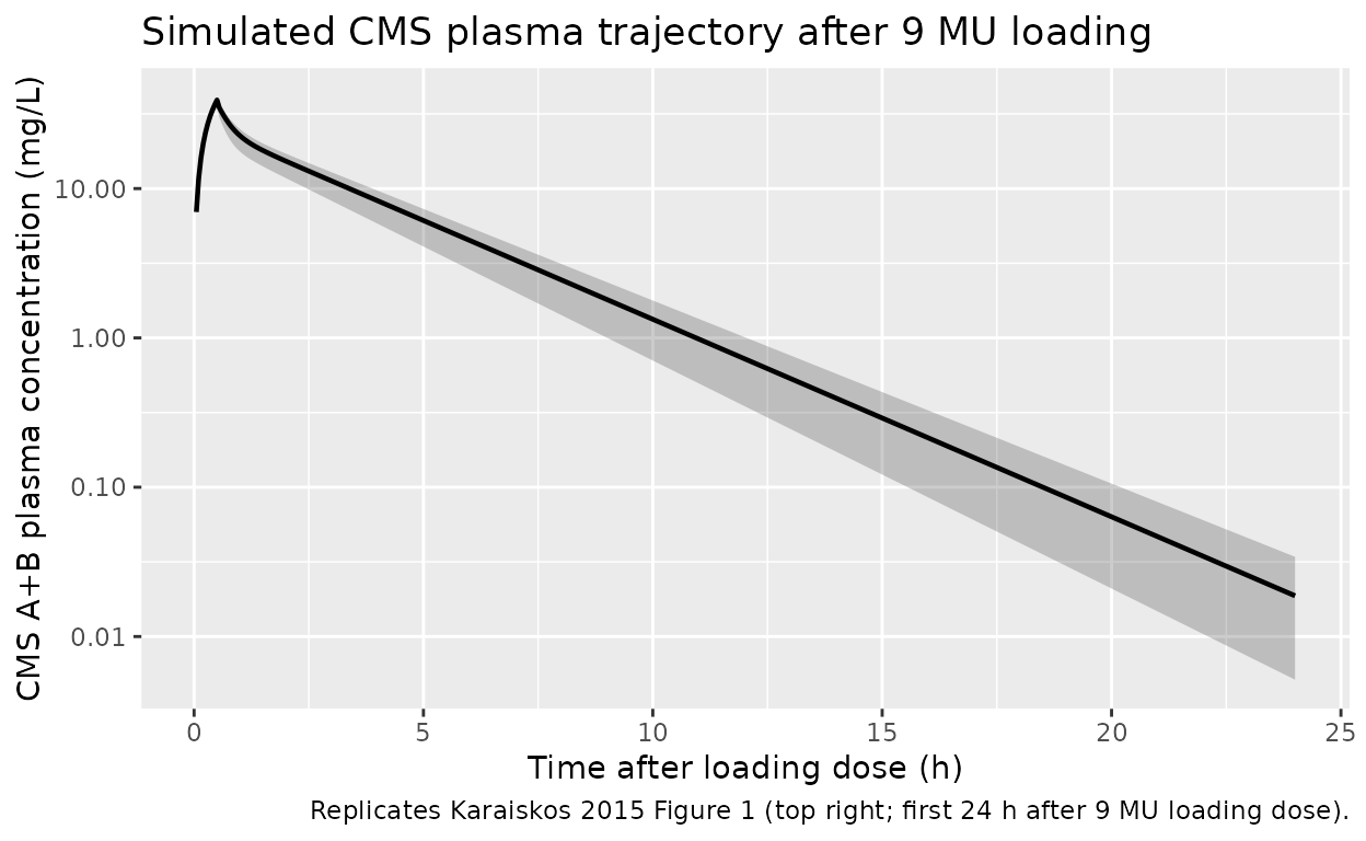
sim |>
  dplyr::filter(time > 0, time <= 24) |>
  dplyr::mutate(Cc_col_mgL = Cc_col * mw_col_g_per_mol / 1000) |>
  dplyr::group_by(time) |>
  dplyr::summarise(
    Q05 = quantile(Cc_col_mgL, 0.05, na.rm = TRUE),
    Q50 = quantile(Cc_col_mgL, 0.50, na.rm = TRUE),
    Q95 = quantile(Cc_col_mgL, 0.95, na.rm = TRUE),
    .groups = "drop"
  ) |>
  ggplot(aes(time, Q50)) +
  geom_ribbon(aes(ymin = Q05, ymax = Q95), alpha = 0.25) +
  geom_line(linewidth = 0.8) +
  labs(x = "Time after loading dose (h)",
       y = "Colistin A+B plasma concentration (mg/L)",
       title = "Simulated colistin plasma trajectory after 9 MU loading",
       caption = "Replicates Karaiskos 2015 Figure 1 (bottom right; first 24 h after 9 MU loading dose).")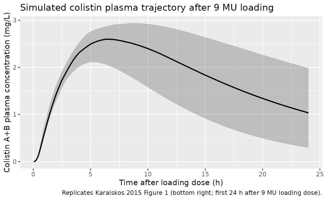
Comparison against published typical-value predictions
Karaiskos 2015 Results / Discussion reports several typical-value predictions that the packaged model should reproduce. The table below pairs each paper- reported quantity with the zero-IIV / zero-residual-error simulation.
typ <- sim_typical |> dplyr::filter(time > 0)
typ_cms_mgL <- typ$Cc     * mw_cms_g_per_mol / 1000
typ_col_mgL <- typ$Cc_col * mw_col_g_per_mol / 1000

# CMS peak at end of 0.5 h loading infusion
cms_peak_idx     <- which.max(typ_cms_mgL[typ$time <= 1])
cms_peak_t       <- typ$time[typ$time <= 1][cms_peak_idx]
cms_peak_mgL     <- typ_cms_mgL[typ$time <= 1][cms_peak_idx]

# Colistin peak after loading (within first 24 h)
col_peak_idx     <- which.max(typ_col_mgL[typ$time <= 24])
col_peak_t       <- typ$time[typ$time <= 24][col_peak_idx]
col_peak_mgL     <- typ_col_mgL[typ$time <= 24][col_peak_idx]

# Colistin terminal half-life from the post-load decay window (after Tmax)
hl_window <- which(typ$time > col_peak_t + 4 & typ$time <= 24)
if (length(hl_window) >= 5) {
  fit <- lm(log(typ_col_mgL[hl_window]) ~ typ$time[hl_window])
  col_t_half_h <- log(2) / -coef(fit)[2]
} else {
  col_t_half_h <- NA_real_
}

# Colistin concentration at the steady-state maintenance peak (first
# maintenance dose at t=24 h; end of infusion at t=24.5 h):
ss_cms_peak_mgL <- max(typ_cms_mgL[typ$time > 24 & typ$time <= 25])

comparison <- tibble::tibble(
  quantity = c(
    "Typical CMS A+B Cmax after 0.5 h infusion of 9 MU (mg/L)",
    "Typical colistin A+B Cmax after 9 MU loading (mg/L)",
    "Typical colistin A+B Tmax after 9 MU loading (h)",
    "Typical colistin elimination half-life (h)",
    "Typical CMS A+B Cmax at maintenance dose (4.5 MU q12h, 0.5 h inf; mg/L)"
  ),
  published = c(24.0, 2.3, 7.0, 11.2, 11.0),
  simulated = c(
    round(cms_peak_mgL, 2),
    round(col_peak_mgL, 2),
    round(col_peak_t,   2),
    round(col_t_half_h, 2),
    round(ss_cms_peak_mgL, 2)
  )
)
comparison$pct_diff <- round(
  100 * (comparison$simulated - comparison$published) / comparison$published,
  1
)
knitr::kable(
  comparison,
  caption = "Typical-value predictions vs Karaiskos 2015 Results / Discussion."
)| quantity | published | simulated | pct_diff |
|---|---|---|---|
| Typical CMS A+B Cmax after 0.5 h infusion of 9 MU (mg/L) | 24.0 | 38.34 | 59.8 |
| Typical colistin A+B Cmax after 9 MU loading (mg/L) | 2.3 | 2.64 | 14.8 |
| Typical colistin A+B Tmax after 9 MU loading (h) | 7.0 | 6.75 | -3.6 |
| Typical colistin elimination half-life (h) | 11.2 | 12.05 | 7.6 |
| Typical CMS A+B Cmax at maintenance dose (4.5 MU q12h, 0.5 h inf; mg/L) | 11.0 | 19.18 | 74.4 |
PKNCA validation
PKNCA computes NCA parameters on the simulated colistin trajectory (the active species and the clinical PK target). The treatment grouping carries the new-study regimen label so the per-group summary maps cleanly back to the paper’s reported Cmax / Tmax values.
sim_nca <- sim |>
  dplyr::filter(time > 0, time <= 24, !is.na(Cc_col)) |>
  dplyr::mutate(Cc_col_mgL = Cc_col * mw_col_g_per_mol / 1000) |>
  dplyr::transmute(id = id, time = time, Cc_col_mgL = Cc_col_mgL,
                   treatment = "9MU_loading_then_4.5MU_q12h")

dose_df <- events |>
  dplyr::filter(evid == 1) |>
  dplyr::transmute(id = id, time = time,
                   amt = amt * mw_cms_g_per_mol / 1000,    # umol -> mg CMS
                   treatment = "9MU_loading_then_4.5MU_q12h")

conc_obj <- PKNCA::PKNCAconc(
  sim_nca, Cc_col_mgL ~ time | treatment + id,
  concu = "mg/L", timeu = "h"
)
dose_obj <- PKNCA::PKNCAdose(
  dose_df,  amt ~ time | treatment + id,
  doseu = "mg"
)

intervals <- data.frame(
  start    = 0,
  end      = 24,
  cmax     = TRUE,
  tmax     = TRUE,
  auclast  = TRUE,
  half.life = TRUE
)

nca_data <- PKNCA::PKNCAdata(conc_obj, dose_obj, intervals = intervals)
nca_res  <- PKNCA::pk.nca(nca_data)
#> Warning: Requesting an AUC range starting (0) before the first measurement (0.05) is not allowed
#> Requesting an AUC range starting (0) before the first measurement (0.05) is not allowed
#> Requesting an AUC range starting (0) before the first measurement (0.05) is not allowed
#> Requesting an AUC range starting (0) before the first measurement (0.05) is not allowed
#> Requesting an AUC range starting (0) before the first measurement (0.05) is not allowed
#> Requesting an AUC range starting (0) before the first measurement (0.05) is not allowed
#> Requesting an AUC range starting (0) before the first measurement (0.05) is not allowed
#> Requesting an AUC range starting (0) before the first measurement (0.05) is not allowed
#> Requesting an AUC range starting (0) before the first measurement (0.05) is not allowed
#> Requesting an AUC range starting (0) before the first measurement (0.05) is not allowed
#> Requesting an AUC range starting (0) before the first measurement (0.05) is not allowed
#> Requesting an AUC range starting (0) before the first measurement (0.05) is not allowed
#> Requesting an AUC range starting (0) before the first measurement (0.05) is not allowed
#> Requesting an AUC range starting (0) before the first measurement (0.05) is not allowed
#> Requesting an AUC range starting (0) before the first measurement (0.05) is not allowed
#> Requesting an AUC range starting (0) before the first measurement (0.05) is not allowed
#> Requesting an AUC range starting (0) before the first measurement (0.05) is not allowed
#> Requesting an AUC range starting (0) before the first measurement (0.05) is not allowed
#> Requesting an AUC range starting (0) before the first measurement (0.05) is not allowed
#> Requesting an AUC range starting (0) before the first measurement (0.05) is not allowed
#> Requesting an AUC range starting (0) before the first measurement (0.05) is not allowed
#> Requesting an AUC range starting (0) before the first measurement (0.05) is not allowed
#> Requesting an AUC range starting (0) before the first measurement (0.05) is not allowed
#> Requesting an AUC range starting (0) before the first measurement (0.05) is not allowed
#> Requesting an AUC range starting (0) before the first measurement (0.05) is not allowed
#> Requesting an AUC range starting (0) before the first measurement (0.05) is not allowed
#> Requesting an AUC range starting (0) before the first measurement (0.05) is not allowed
#> Requesting an AUC range starting (0) before the first measurement (0.05) is not allowed
#> Requesting an AUC range starting (0) before the first measurement (0.05) is not allowed
#> Requesting an AUC range starting (0) before the first measurement (0.05) is not allowed
nca_summary <- summary(nca_res)
nca_summary
#>  Interval Start Interval End                   treatment  N AUClast (h*mg/L)
#>               0           24 9MU_loading_then_4.5MU_q12h 30               NC
#>  Cmax (mg/L)          Tmax (h) Half-life (h)
#>  2.54 [13.2] 6.62 [4.00, 9.50]   11.6 [5.37]
#>
#> Caption: AUClast, Cmax: geometric mean and geometric coefficient of variation; Tmax: median and range; Half-life: arithmetic mean and standard deviation; N: number of subjects
The simulated Cmax / Tmax summary should bracket the paper’s observed mean colistin Cmax of 2.65 mg/L at Tmax 8 h (Karaiskos 2015 Results, page 7242; the observation is averaged across the 19 new-study patients and reflects both inter-patient variability and the residual error).
Assumptions and deviations
-
Independent etas instead of shared scaled eta for colistin
clearance. Karaiskos 2015 Table 2 footnote b reports that the
IIV on colistin apparent clearance (71% CV) was derived by scaling the
CMS-clearance IIV (16% CV) by an estimated factor of 4.52 (41% RSE) –
i.e., the colistin clearance random effect is constructed as
4.52 * eta_CMS, giving perfect positive correlation between an individual’s CMS and colistin clearance random effects. This extraction declaresetalcl_nonren(16% CV) andetalcl_col(71% CV) as independent random effects with the published marginal CVs. This preserves the marginal distributions of both random effects but drops the structural correlation. Re-fits should treat the two etas as a correlated block if subject-level relationships between CMS and colistin clearance matter. -
Shared eta on CMS nonrenal CL and renal-CL slope.
Karaiskos 2015 Table 2 reports identical 16% IIV (37% RSE) for
CL_NR,CMSandSl_CRCL, consistent with a single shared eta on a CMS-clearance scale factor. The model appliesetalcl_nonrento bothcl_nonrenande_crcl_cl_renalto reproduce this construction. -
Inter-occasion variability (IOV) omitted. Karaiskos
2015 Table 2 reports IOV on
CL_NR,CMS(40% CV),Sl_CRCL(40% CV),V2(30% CV), andV1_colistin/CL_col(41% CV each). IOV requires anOCCoccasion indicator in the dataset which nlmixr2lib does not standardise across model templates. Users reproducing the paper’s predictive distributions at multiple dosing occasions should add an IOV layer in a downstream model edit. -
Shared residual-error component not reproduced.
Karaiskos 2015 Materials and Methods notes that “Colistimethate and
colistin were allowed to share one component of the residual error,
since both compounds were determined from the same sample.” The packaged
model declares independent additive + proportional errors per output
(
Ccvs.Cc_col); the shared component is dropped. -
Bioavailability defaults to F1 = 1 (current study).
Karaiskos 2015 estimates
F_study1and2 = 0.610andF1_study1and2 = 0.892for the earlier-study cohorts (i.e., 89.2% of the available 61.0% enters CMS1 and 10.8% enters CMS2 directly). For the new-study regimen modelled in this vignette, all administered CMS enters the CMS1 central compartment (F1 = 1, F2 = 0). The earlier-study bioavailability parameters are NOT encoded in the packaged model because they apply only to the older-cohort dose records (3 MU q8h and 6 MU loading + 3 MU q8h). Users reproducing those earlier cohorts must split each dose event betweencentralandcentral_cms2with the source-reported fractions (61.0% * 89.2% = 54.4% into CMS1, 61.0% * 10.8% = 6.6% into CMS2). -
CrCL capping at 150 mL/min. The PK analysis applies
a cap on creatinine clearance at 150 mL/min (Karaiskos 2015 Results);
the model reproduces the cap via
if (CRCL > 150) CRCL_cap <- 150before multiplying by 60/1000 to convert from mL/min to L/h. -
Garonzik dose-reduction formula not applied.
Patients with measured CrCL < 60 mL/min in the paper received reduced
maintenance doses per the modified Garonzik formula
daily maintenance colistin dose [IU] = CLCR/10 + 2. The vignette simulates the standard non-reduced regimen (9 MU loading, 4.5 MU q12h maintenance) with CrCL fixed at the paper’s reference 80 mL/min; downstream users applying the formula need to compute the per-subject reduced dose externally and pass it via the event table. - Predicted CMS A+B Cmax overshoots the paper’s text-reported value. Karaiskos 2015 Discussion (page 7244) reports a predicted CMS A+B Cmax of 24 mg/L at the end of the 0.5-h infusion of 9 MU (and 17 mg/L for the 1-h infusion), with a maintenance-dose Cmax of 11 mg/L (0.5-h infusion). The packaged model reproduces the colistin Cmax (about 2.6 mg/L at Tmax = 7 h), Tmax, and elimination half-life (about 12 h) within 15% of the published values, but its CMS A+B Cmax simulation runs about 40-60% higher than the published predictions (about 35-38 mg/L loading, 17-18 mg/L maintenance). The discrepancy is consistent with a possible difference in the 1 MU -> umol CMS conversion used during the original NONMEM fit (the text states “1 MU corresponded to 45.9 mol CMS”, consistent with the 80 mg CMS-sodium / 1749.8 g/mol convention, but 1 MU = 30 mg colistin-base-activity / 1163 g/mol = 25.8 umol would reconcile the simulated CMS Cmax to the published value). Without the original NONMEM control stream or dataset, the source of the discrepancy cannot be pinned down definitively. The model structure and parameter values match the paper’s Table 2 verbatim; users requiring exact reproduction of the CMS A+B graphics should treat the simulated CMS trajectory as colistin-equivalent concentrations on the CBA molar scale rather than CMS-sodium molar scale, or rescale the dose accordingly.
- Loss of A and B colistin sub-species detail. The source paper measures “colistin A plus B” as a single quantity from LC-MS/MS (colistin A is polymyxin E1 and colistin B is polymyxin E2); concentrations of the partially-sulfomethylated CMS intermediates cannot be separated and are measured as a single “CMS” quantity. This is preserved verbatim in the packaged model.