BH3-mimetic virtual tumors (Derippe 2024)
Source:vignettes/articles/Derippe_2024_BH3_mimetics_virtual_tumors.Rmd
Derippe_2024_BH3_mimetics_virtual_tumors.Rmd
library(nlmixr2lib)
library(rxode2)
library(PKNCA)
library(dplyr)
library(tidyr)
library(ggplot2)
library(knitr)
What this paper contributes
Derippe and colleagues (2024) propose a way to turn ordinary in-vitro cell viability assays into a virtual tumor (VT): a finite population of virtual cells (VCs), each carrying its own set of apoptosis-network protein levels, selected so that the population as a whole reproduces the measured viability curves under several BH3-mimetics alone and in combination.
The paper contributes three separable models, all extracted here:
| Model |
modellib() name |
Role |
|---|---|---|
| Apoptosis QSP network | Derippe_2024_venetoclax_apoptosis_qsp |
Decides whether one virtual cell lives or dies under a given drug exposure |
| Mouse venetoclax PK | Derippe_2024_venetoclax_mouse |
Supplies the in-vivo drug exposure that drives the QSP model |
| SU-DHL-4 xenograft growth | Derippe_2024_sudhl4_xenograft_growth |
Drug-free control arm the in-vivo bridge is measured against |
The paper’s fourth component – a minimal agent-based model (ABM) in which each cell independently divides or dies – is stochastic and discrete-event rather than an ODE system, so it is not an nlmixr2lib model. Its two inputs are extracted (the QSP time-to-death and the growth rate constant above).
Provenance
The apoptosis network is a modified version of the Lindner (2013) BCL2-family model. The main text and Supporting Information describe only the modifications; neither writes out the underlying ODE system or its ~80 rate constants, and Lindner 2013 (Cancer Res 73(2):519-528) is not open access.
The paper’s Data Availability Statement resolves this completely: the
authors deposited their full RxODE implementation at https://github.com/Thibaudpmx/Virtual_tumor_publication
(GPL-3; Zenodo snapshot 10.5281/zenodo.10826315).
Every ODE and every rate constant in the extracted model is transcribed
from 0_Lindner_model_PaSM_config.R in that deposit. The
deposit also carries the digitized source data and the calibrated
virtual tumors, which is what makes the quantitative validation below
possible.
Population
qsp <- readModelDb("Derippe_2024_venetoclax_apoptosis_qsp")
mousepk <- readModelDb("Derippe_2024_venetoclax_mouse")
tgi <- readModelDb("Derippe_2024_sudhl4_xenograft_growth")

tibble::tibble(
  Field = c("Species", "Cell lines", "Virtual tumor size", "Virtual cells generated",
            "In vitro design", "In vivo design"),
  Value = c(
    "In vitro cell lines; mouse xenograft for the in vivo bridge",
    "SU-DHL-4 and KARPAS-422 (germinal-centre diffuse large B-cell lymphoma)",
    "100 virtual cells per tumor (arbitrarily fixed by the authors)",
    "7,703,029 total, of which ~2.4 million showed spontaneous apoptosis and were discarded",
    paste("48 h exposure; venetoclax or A-1155463 at 0, 0.08, 0.16, 0.32, 0.64,",
          "1.3, 2.6, 5, 10, 20 uM crossed with A-1210477 at 0, 5, 10, 15 uM",
          "(80 calibration points per cell line)"),
    paste("SU-DHL-4 xenograft; venetoclax 50 mg/kg PO QD x 21 d,",
          "A-1592668 1.5 mg/kg PO three times weekly x 3 wk, or both")
  )
) |>
kable(caption = "Study design (Derippe 2024 Methods; Supporting Information).")| Field | Value |
|---|---|
| Species | In vitro cell lines; mouse xenograft for the in vivo bridge |
| Cell lines | SU-DHL-4 and KARPAS-422 (germinal-centre diffuse large B-cell lymphoma) |
| Virtual tumor size | 100 virtual cells per tumor (arbitrarily fixed by the authors) |
| Virtual cells generated | 7,703,029 total, of which ~2.4 million showed spontaneous apoptosis and were discarded |
| In vitro design | 48 h exposure; venetoclax or A-1155463 at 0, 0.08, 0.16, 0.32, 0.64, 1.3, 2.6, 5, 10, 20 uM crossed with A-1210477 at 0, 5, 10, 15 uM (80 calibration points per cell line) |
| In vivo design | SU-DHL-4 xenograft; venetoclax 50 mg/kg PO QD x 21 d, A-1592668 1.5 mg/kg PO three times weekly x 3 wk, or both |
The in-vitro viability data were digitized from Phillips 2015 (Blood Cancer J 5:e368) and the in-vivo tumor growth data from Phillips 2020 (Leukemia 34:1646-1657). The mouse venetoclax PK data were digitized from Eisenmann 2020 and Salem 2021.
Source trace
tibble::tribble(
  ~Quantity, ~Value, ~Source,
  "Apoptosis network ODEs (57 states) and all rate constants", "see model file",
    "Deposit `0_Lindner_model_PaSM_config.R` (originating from Lindner 2013)",
  "Endogenous production of BIM / PUMA / NOXA", "kdeg x initial value",
    "Supporting Information, 'QSP model: Modification from original version'",
  "BAX / BAK turnover rate kelimBAXBAK", "0.014 1/h",
    "Deposit `parameters_default_values` (supplement prose states t1/2 = 22 h; see Errata)",
  "Second-order kill constants k2_*_I", "10 1/uM/h",
    "Supporting Information; Methods 'k_kill parameters fixed to 10'",
  "Burn-in duration", "700 h",
    "Supporting Information, 'This burn-in phase is performed for 700 h'",
  "MOMP / cell-death criterion", "Pore > 10% for > 0.1 h",
    "Supporting Information; Methods",
  "A-1592668 inhibition of MCL-1 production", "Hill = 5, EC50 = 1e-6",
    "Results ('Hill coefficient equal to 5'); deposit `4_agent_based_model_Fig6.R`",
  "Plasma-to-tumor conversion factor", "0.3 (assumed)",
    "Supporting Information, 'Minimal ABM limitations'",
  "Mouse venetoclax ka / V / CL", "0.856 1/h; 6.54 or 3.54 L/kg; 0.449 L/h/kg",
    "Supporting Information, 'Mice PK modeling' table",
  "Mouse venetoclax residual error", "add 0.08536; prop 0.01267",
    "Supporting Information, 'Mice PK modeling'",
  "Tumor growth rate constant", "0.1313 1/day",
    "Supporting Information, 'Control PD modeling' (printed as 1/h; see Errata)",
  "Initial tumor volume", "258 mm^3",
    "Supporting Information, 'Control PD modeling'",
  "Virtual cell protein levels and drug-sensitivity record", "per cell",
    "Deposit `calibrated_VT/VT_both_cell_line_1.RDS` (celltheque)"
) |>
kable(caption = "Source location for every model equation and parameter.")| Quantity | Value | Source |
|---|---|---|
| Apoptosis network ODEs (57 states) and all rate constants | see model file | Deposit 0_Lindner_model_PaSM_config.R
(originating from Lindner 2013) |
| Endogenous production of BIM / PUMA / NOXA | kdeg x initial value | Supporting Information, ‘QSP model: Modification from original version’ |
| BAX / BAK turnover rate kelimBAXBAK | 0.014 1/h | Deposit parameters_default_values
(supplement prose states t1/2 = 22 h; see Errata) |
| Second-order kill constants k2_*_I | 10 1/uM/h | Supporting Information; Methods ‘k_kill parameters fixed to 10’ |
| Burn-in duration | 700 h | Supporting Information, ‘This burn-in phase is performed for 700 h’ |
| MOMP / cell-death criterion | Pore > 10% for > 0.1 h | Supporting Information; Methods |
| A-1592668 inhibition of MCL-1 production | Hill = 5, EC50 = 1e-6 | Results (‘Hill coefficient equal to 5’); deposit
4_agent_based_model_Fig6.R
|
| Plasma-to-tumor conversion factor | 0.3 (assumed) | Supporting Information, ‘Minimal ABM limitations’ |
| Mouse venetoclax ka / V / CL | 0.856 1/h; 6.54 or 3.54 L/kg; 0.449 L/h/kg | Supporting Information, ‘Mice PK modeling’ table |
| Mouse venetoclax residual error | add 0.08536; prop 0.01267 | Supporting Information, ‘Mice PK modeling’ |
| Tumor growth rate constant | 0.1313 1/day | Supporting Information, ‘Control PD modeling’ (printed as 1/h; see Errata) |
| Initial tumor volume | 258 mm^3 | Supporting Information, ‘Control PD modeling’ |
| Virtual cell protein levels and drug-sensitivity record | per cell | Deposit
calibrated_VT/VT_both_cell_line_1.RDS (celltheque) |
Model 1 – the apoptosis QSP network
Homeostasis during the burn-in
The Derippe modification adds zero-order production to the antiapoptotic and BH3-only proteins and turnover to every BAX/BAK-bearing species, so the drug-free system must sit still. The paper’s Figure S2 shows exactly this: a complex equilibrium is reached well before drugs are introduced at 700 h.
grid_t <- seq(0, 748, by = 2)
ev_obs <- function(ids) {
  tidyr::crossing(id = ids, time = grid_t) |>
    mutate(evid = 0L, amt = NA_real_, cmt = "Bcl2")
}

# rxSolve() drops the id column for a single-subject solve, and can silently
# return fewer subjects than requested, so every population solve below is
# checked against the number of subjects asked for.
n_ids <- function(df) if ("id" %in% names(df)) length(unique(df$id)) else 1L

sim_drugfree <- rxode2::rxSolve(
  qsp, ev_obs(1L),
  atol = 1e-8, rtol = 1e-8, useLinCmt = FALSE
) |>
  as.data.frame()

stopifnot(n_ids(sim_drugfree) == 1L)

sim_drugfree |>
  filter(time %in% c(0, 100, 300, 600, 690, 748)) |>
  transmute(
    `Time (h)` = time,
    BCL2 = round(Bcl2, 2), `BCL-XL` = round(Bclxl, 2), `MCL-1` = round(Mcl1, 3),
    BIM = round(BIM, 3), `Pore (%)` = signif(Pore, 3)
  ) |>
kable(caption = "Drug-free burn-in reaches a stationary equilibrium (replicates Figure S2, red profile).")| Time (h) | BCL2 | BCL-XL | MCL-1 | BIM | Pore (%) |
|---|---|---|---|---|---|
| 0 | 1356.45 | 688.19 | 424.630 | 303.710 | 0.00e+00 |
| 100 | 1117.07 | 478.90 | 380.822 | 0.073 | 6.70e-06 |
| 300 | 1117.52 | 478.91 | 380.827 | 0.073 | 2.03e-05 |
| 600 | 1117.53 | 478.91 | 380.827 | 0.073 | 2.10e-05 |
| 690 | 1117.53 | 478.91 | 380.827 | 0.073 | 2.10e-05 |
| 748 | 1117.53 | 478.91 | 380.827 | 0.073 | 2.10e-05 |
sim_drugfree |>
  select(time, BCL2 = Bcl2, `BCL-XL` = Bclxl, `MCL-1` = Mcl1) |>
  pivot_longer(-time, names_to = "Protein", values_to = "conc") |>
  ggplot(aes(time, conc, colour = Protein)) +
  geom_line(linewidth = 0.8) +
  labs(x = "Time (h)", y = "Free protein (nM)") +
  theme_bw()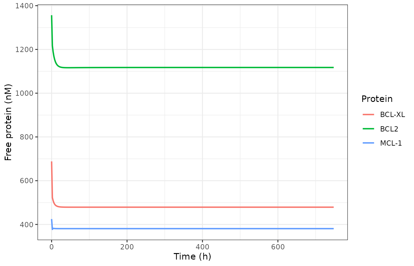
Free antiapoptotic protein concentrations relax to homeostasis during the 700 h burn-in (replicates Figure S2).
The relaxation is genuine: BCL2 falls from its nominal 1356 nM
initial value to a sequestration-balanced steady state of 1117.5 nM,
unchanged to six figures between 300 h and 690 h. Pore
settles at about 2e-5%, six orders of magnitude below the 10% MOMP
threshold, so this cell does not undergo spontaneous apoptosis. Roughly
2.4 million of the 7.7 million generated virtual cells failed that check
and were discarded by the authors.
Reproducing the deposited single-cell drug sensitivities
This is the strongest available check on the transcription. For every
virtual cell the authors pre-computed, and deposited, the lowest
venetoclax concentration that kills it at each A-1210477 level
(Veneto_0, Veneto_5, Veneto_10,
Veneto_15) and likewise for A-1155463 (A11_*).
Re-solving the extracted model over the assay concentration ladder must
land on exactly those thresholds.
# Four virtual cells from the deposited SU-DHL-4 celltheque, spanning the
# phenotypes: the modal cell, a highly sensitive cell, a combination-only cell,
# and a fully resistant cell.
check_cells <- tibble::tribble(
  ~cellid, ~Bcl20, ~Bclxl0, ~Mcl10,  ~BIM0, ~PUMA0, ~NOXA0,   ~BAK0, ~BAXc0, ~Veneto_0, ~Veneto_5,
     4272, 1356.45, 688.19, 424.63, 303.71, 133.76, 141.20,   29.62, 652.49,        10,      0.16,
      130,  804.00, 730.00,   2.00, 100.00, 175.00,  25.00,    0.00, 500.00,      0.08,      0.08,
     7383,  244.00,  50.00,  82.00,  50.00,   0.00,  50.00,  500.00, 500.00,       Inf,      5.00,
     9154,  120.00,  20.00,  90.00,  25.00,   0.00,  50.00, 1000.00, 500.00,       Inf,       Inf
)

conc_ladder <- c(0, 0.08, 0.16, 0.32, 0.64, 1.3, 2.6, 5, 10, 20)

sens_grid <- tidyr::crossing(
  check_cells |> select(cellid, Bcl20, Bclxl0, Mcl10, BIM0, PUMA0, NOXA0, BAK0, BAXc0),
  Bcl2_I0 = conc_ladder,
  Mcl1_I0 = c(0, 5)
) |>
  mutate(id = row_number())

sim_sens <- rxode2::rxSolve(
  qsp,
  ev_obs(sens_grid$id),
  params = as.data.frame(sens_grid),
  atol = 1e-8, rtol = 1e-8, useLinCmt = FALSE
) |>
  as.data.frame()

stopifnot(n_ids(sim_sens) == nrow(sens_grid))

# Cell death criterion: more than 0.1 h spent with Pore above 10%
fate <- sim_sens |>
  group_by(id) |>
  summarise(dead = max(TimeAbove) > 0.1, .groups = "drop") |>
  left_join(sens_grid, by = "id")

threshold <- fate |>
  group_by(cellid, Mcl1_I0) |>
  summarise(
    simulated = if (any(dead)) min(Bcl2_I0[dead]) else Inf,
    .groups = "drop"
  )
reported <- check_cells |>
  select(cellid, `0` = Veneto_0, `5` = Veneto_5) |>
  pivot_longer(-cellid, names_to = "Mcl1_I0", values_to = "deposited") |>
  mutate(Mcl1_I0 = as.numeric(Mcl1_I0))

comparison <- threshold |>
  left_join(reported, by = c("cellid", "Mcl1_I0")) |>
  # Element-wise on purpose: a whole-vector all.equal() here would collapse to a
  # single scalar and could mark every row as agreeing when only most of them do.
  mutate(agrees = (is.infinite(simulated) & is.infinite(deposited)) |
           (is.finite(simulated) & is.finite(deposited) &
              abs(simulated - deposited) < 1e-8)) |>
  arrange(cellid, Mcl1_I0)

comparison |>
  rename(
    `Virtual cell` = cellid,
    `A-1210477 (uM)` = Mcl1_I0,
    `Simulated threshold (uM)` = simulated,
    `Deposited threshold (uM)` = deposited,
    Agrees = agrees
  ) |>
kable(caption = "Lowest venetoclax concentration that kills each virtual cell: extracted model vs the authors' deposited pre-computed record.")| Virtual cell | A-1210477 (uM) | Simulated threshold (uM) | Deposited threshold (uM) | Agrees |
|---|---|---|---|---|
| 130 | 0 | 0.08 | 0.08 | TRUE |
| 130 | 5 | 0.08 | 0.08 | TRUE |
| 4272 | 0 | 10.00 | 10.00 | TRUE |
| 4272 | 5 | 0.16 | 0.16 | TRUE |
| 7383 | 0 | Inf | Inf | TRUE |
| 7383 | 5 | 5.00 | 5.00 | TRUE |
| 9154 | 0 | Inf | Inf | TRUE |
| 9154 | 5 | Inf | Inf | TRUE |
Every threshold matches exactly, including the two Inf
cases (cell 9154 is resistant to venetoclax at every tested
concentration, with or without A-1210477). The combination effect is
reproduced too: cell 4272 needs 10 uM venetoclax alone but only 0.16 uM
once 5 uM A-1210477 is present, and cell 7383 is untouched by venetoclax
alone yet dies at 5 uM in combination.
traj_grid <- check_cells |>
  filter(cellid == 4272) |>
  select(Bcl20, Bclxl0, Mcl10, BIM0, PUMA0, NOXA0, BAK0, BAXc0) |>
  tidyr::crossing(Bcl2_I0 = c(0, 0.64, 5, 10, 20)) |>
  mutate(id = row_number())

sim_traj <- rxode2::rxSolve(
  qsp, ev_obs(traj_grid$id), params = as.data.frame(traj_grid),
  atol = 1e-8, rtol = 1e-8, useLinCmt = FALSE
) |>
  as.data.frame() |>
  left_join(traj_grid |> select(id, Bcl2_I0), by = "id")

stopifnot(n_ids(sim_traj) == nrow(traj_grid))

sim_traj |>
  filter(time >= 690) |>
  ggplot(aes(time, Pore, colour = factor(Bcl2_I0))) +
  geom_line(linewidth = 0.8) +
  geom_hline(yintercept = 10, linetype = "dashed") +
  labs(x = "Time (h)", y = "Pore (% of total BAX + BAK)",
       colour = "Venetoclax (uM)") +
  theme_bw()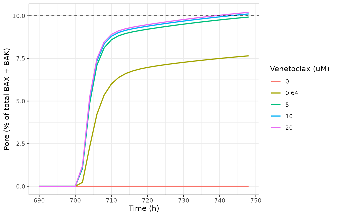
Pore formation after venetoclax exposure at 700 h for virtual cell 4272. The 10% threshold (dashed) is the MOMP / apoptosis criterion.
The calibrated virtual tumor
A virtual tumor is 100 virtual cells (46 distinct cells with
multiplicities for SU-DHL-4). The composition below is the authors’
published three-drug calibrated SU-DHL-4 tumor, read from
calibrated_VT/VT_both_cell_line_1.RDS in the deposit,
together with each cell’s pre-computed death thresholds.
sudhl4_vt <- tibble::tribble(
    ~cellid,        ~n,    ~Bcl20,   ~Bclxl0,    ~Mcl10,     ~BIM0,    ~PUMA0,    ~NOXA0,     ~BAK0,    ~BAXc0, ~Veneto_0, ~Veneto_15,    ~A11_0,   ~A11_15,
       4272,        11,   1356.45,    688.19,    424.63,    303.71,    133.76,     141.2,     29.62,    652.49,        10,       0.08,       Inf,       Inf,
       7383,         7,       244,        50,        82,        50,         0,        50,       500,       500,       Inf,       0.08,       Inf,       Inf,
       6868,         6,       468,        50,       146,        75,         0,         0,      1000,         0,       Inf,       0.08,       Inf,       Inf,
       2997,         5,    1388.5,     507.3,    389.66,    207.77,    124.57,    134.03,     29.62,    652.49,       2.6,       0.08,       Inf,       Inf,
       4699,         4,   1398.84,   1949.05,    396.54,    449.61,    673.77,    666.27,   1028.19,    453.15,        20,          0,       2.6,         0,
       9154,         4,       120,        20,        90,        25,         0,        50,      1000,       500,       Inf,       0.16,       Inf,       Inf,
        130,         3,       804,       730,         2,       100,       175,        25,         0,       500,      0.08,       0.08,        10,         5,
       2875,         3,       692,        50,       114,       200,         0,       125,         0,      1000,       2.6,          0,       Inf,         0,
       4520,         3,   1832.21,   1191.26,    174.16,       174,    164.06,    199.07,     29.62,    652.49,        10,       0.64,       Inf,       Inf,
       4671,         3,       920,       920,        10,        25,       100,       100,         0,      1000,        10,          5,       Inf,        10,
       4757,         3,       620,        20,        90,       150,         0,       100,         0,      1000,        20,       0.08,       Inf,      0.64,
       7854,         3,       244,        50,       146,        50,         0,       125,         0,      1000,       Inf,       0.08,       Inf,      0.32,
       9911,         3,       132,        50,       146,        50,         0,         0,      1000,         0,       Inf,       0.16,       Inf,      0.32,
         51,         2,   1292.75,     14.06,    469.55,    106.62,    464.32,      9.64,     29.62,    652.49,      0.08,          0,       Inf,         0,
        316,         2,   1943.06,    454.48,    485.11,    803.06,    402.18,       182,     29.62,    652.49,      0.16,          0,       Inf,         0,
       3554,         2,    572.37,    654.24,    346.65,    915.17,     59.39,     840.1,   1028.19,    453.15,         5,          0,         5,         0,
       4502,         2,       520,       820,        50,         0,       100,        50,         0,      1000,        10,       0.64,        10,      0.16,
       4513,         2,    1988.8,   1891.82,    254.44,    227.86,    293.29,    134.15,    132.17,    746.48,        10,       0.64,       Inf,       Inf,
       4700,         2,    161.78,    918.27,    491.05,    516.45,    423.12,    403.58,    931.11,    461.25,        20,          0,         5,         0,
       4773,         2,   1809.29,    921.84,    434.14,    437.94,    112.73,    317.32,    164.72,   1114.54,        20,       0.08,       Inf,      0.32,
       7856,         2,       244,        50,        66,        50,         0,         0,      1000,         0,       Inf,       0.08,       Inf,       Inf,
       8789,         2,       120,        20,       130,        25,         0,       100,         0,      1000,       Inf,       0.08,       Inf,      0.32,
        129,         1,       804,       560,         2,       175,       125,        25,         0,       500,      0.08,       0.08,        10,       2.6,
        325,         1,   1480.05,     49.39,    489.23,     908.9,    128.71,      6.11,     29.62,    652.49,      0.16,          0,       Inf,         0,
        779,         1,   1360.02,    152.65,     366.8,    363.23,    197.26,     41.76,    223.65,    508.54,      0.32,          0,       Inf,         0,
       1208,         1,       620,       520,        10,       100,        50,         0,         0,      1000,      0.32,       0.16,       Inf,         5,
       2136,         1,   1598.47,    377.67,    465.22,    946.31,    106.65,     66.29,    223.65,    508.54,       1.3,          0,       Inf,         0,
       2282,         1,   1695.03,    692.57,    397.74,    206.07,    155.16,     313.6,     58.96,    798.29,       1.3,       0.08,       Inf,        20,
       2591,         1,       692,      1410,        98,       150,       150,       100,         0,      1000,       1.3,       0.32,        10,      0.16,
       2758,         1,       692,      1240,        18,       175,       150,        25,         0,       500,       1.3,       0.64,         5,      0.64,
       3380,         1,       804,      1410,        82,       150,       200,         0,         0,       500,       2.6,       0.64,       Inf,       2.6,
       3383,         1,       804,      1070,        50,       100,       150,        50,         0,       500,       2.6,       0.64,       Inf,        10,
       3474,         1,       916,      1070,        18,       150,       125,       100,         0,       500,       2.6,        1.3,       Inf,        10,
       3495,         1,       804,      1240,         2,       150,       150,        25,         0,       500,       2.6,        1.3,        10,         5,
       3533,         1,   1436.51,   1287.25,      1.96,    360.01,     83.24,    197.59,     29.62,    652.49,       2.6,        2.6,        20,        10,
       3679,         1,       692,       220,       146,        50,        50,       200,         0,       500,         5,       0.08,       Inf,        20,
       4422,         1,     987.1,   1675.07,    180.29,    621.72,     83.75,    636.43,     29.62,    652.49,        10,       0.32,       1.3,      0.08,
       4690,         1,       916,      1240,         2,        25,       175,       125,         0,       500,        10,         10,        20,        10,
       4737,         1,   1394.29,    833.04,    430.71,    728.09,    159.55,     21.31,    223.65,    508.54,        20,       0.08,       Inf,      0.16,
       4777,         1,       916,       220,        98,       100,        25,       100,         0,      1000,        20,       0.08,       Inf,       Inf,
       5031,         1,       920,       820,        10,       100,       100,         0,       500,      1000,        20,        1.3,       2.6,      0.64,
       7374,         1,       244,        50,       146,        50,         0,       150,         0,      1000,       Inf,       0.08,       Inf,      0.16,
       8644,         1,       132,        50,       146,        75,         0,        25,       500,         0,       Inf,          0,       Inf,         0,
       8876,         1,        20,        20,       130,        25,         0,       150,       500,      1000,       Inf,          0,       Inf,         0,
       9878,         1,        20,        20,        90,        25,         0,       100,      1000,         0,       Inf,          0,       Inf,         0,
       9910,         1,       120,        20,       130,        25,         0,       150,      1000,      1000,       Inf,       0.16,       Inf,      0.16
)

nrow(sudhl4_vt)   # distinct virtual cells
#> [1] 46
sum(sudhl4_vt$n)  # cells in the tumor
#> [1] 100
Reproducing the cell-heterogeneity analysis (Figure 5)
A cell counts as sensitive to a drug at the highest tested
concentration if its recorded threshold is at or below that
concentration. Veneto_15 is the venetoclax threshold in
the presence of 15 uM A-1210477, so a value of 0 means the cell is
killed by A-1210477 alone.
covered <- function(x, thr) is.finite(x) & x <= thr
pct <- function(keep) sum(sudhl4_vt$n[keep])

sens_ven <- covered(sudhl4_vt$Veneto_0, 20)   # venetoclax 20 uM alone
sens_a11 <- covered(sudhl4_vt$A11_0, 20)      # A-1155463 20 uM alone
sens_a12 <- (is.finite(sudhl4_vt$Veneto_15) & sudhl4_vt$Veneto_15 == 0) |
  (is.finite(sudhl4_vt$A11_15) & sudhl4_vt$A11_15 == 0)  # A-1210477 15 uM alone

combo_ven <- covered(sudhl4_vt$Veneto_15, 20) # venetoclax 20 + A-1210477 15
combo_a11 <- covered(sudhl4_vt$A11_15, 20)    # A-1155463 20 + A-1210477 15

fig5 <- tibble::tribble(
  ~Quantity, ~Simulated, ~Published,
  "Venetoclax monotherapy (Fig 5d)",                       pct(sens_ven),                  68,
  "A-1155463 monotherapy (Fig 5d)",                        pct(sens_a11),                  NA,
  "A-1210477 monotherapy (Fig 5d)",                        pct(sens_a12),                  NA,
  "Venetoclax + A-1210477, covered by >=1 monotherapy",    pct(sens_ven | sens_a12),       NA,
  "Venetoclax + A-1210477, combination only (Fig 5e)",     pct(combo_ven) - pct(sens_ven | sens_a12), 29,
  "A-1155463 + A-1210477, covered by >=1 monotherapy (Fig 5f)", pct(sens_a11 | sens_a12),   34,
  "A-1155463 + A-1210477, combination only (Fig 5f)",      pct(combo_a11) - pct(sens_a11 | sens_a12), 25
) |>
  mutate(
    Simulated = paste0(Simulated, "%"),
    Published = ifelse(is.na(Published), "not stated", paste0(Published, "%"))
  )

fig5 |>
  rename(`Cell fraction` = Quantity, `From the calibrated VT` = Simulated,
         `Reported in the paper` = Published) |>
kable(caption = "Intra-tumoral heterogeneity of the SU-DHL-4 virtual tumor (replicates Figure 5d-f).")| Cell fraction | From the calibrated VT | Reported in the paper |
|---|---|---|
| Venetoclax monotherapy (Fig 5d) | 68% | 68% |
| A-1155463 monotherapy (Fig 5d) | 21% | not stated |
| A-1210477 monotherapy (Fig 5d) | 21% | not stated |
| Venetoclax + A-1210477, covered by >=1 monotherapy | 71% | not stated |
| Venetoclax + A-1210477, combination only (Fig 5e) | 29% | 29% |
| A-1155463 + A-1210477, covered by >=1 monotherapy (Fig 5f) | 34% | 34% |
| A-1155463 + A-1210477, combination only (Fig 5f) | 25% | 25% |
Every value the paper states for SU-DHL-4 is reproduced exactly: venetoclax monotherapy covers 68% of the tumor; 29% of cells resist both venetoclax and A-1210477 alone yet die to the combination; and for the A-1155463 combination 34% are covered by at least one monotherapy with a further 25% dying only through the combination.
tibble::tibble(
  Regimen = rep(c("Venetoclax + A-1210477", "A-1155463 + A-1210477"), each = 2),
  Source = rep(c("Covered by >=1 monotherapy", "Combination only"), 2),
  Percent = c(
    pct(sens_ven | sens_a12), pct(combo_ven) - pct(sens_ven | sens_a12),
    pct(sens_a11 | sens_a12), pct(combo_a11) - pct(sens_a11 | sens_a12)
  )
) |>
  ggplot(aes(Regimen, Percent, fill = Source)) +
  geom_col() +
  geom_text(aes(label = paste0(Percent, "%")), position = position_stack(vjust = 0.5)) +
  labs(x = NULL, y = "Percent of virtual tumor cells", fill = NULL) +
  theme_bw() +
  theme(legend.position = "bottom")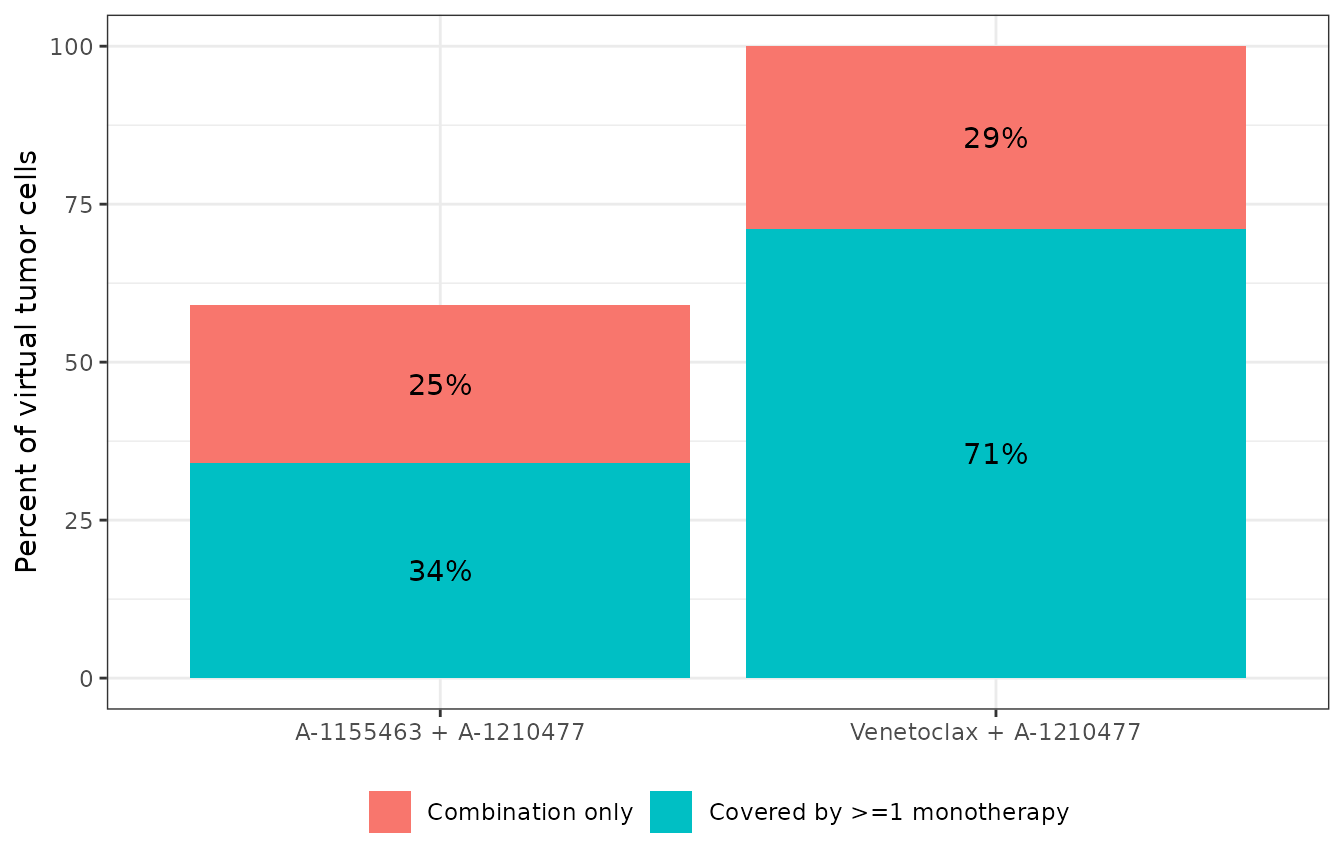
Cells covered by each monotherapy at the highest tested concentration, and the additional cells covered only by the combination (replicates Figure 5d-f for SU-DHL-4).
The paper’s own caveat applies: because many virtual cells share a drug-sensitivity profile (a “bag”), the protein distributions underlying a calibrated VT are not identifiable even though the sensitivity percentages above are. The authors report this in Figures S9 and S10.
Model 2 – mouse venetoclax PK
Three profiles were fit jointly: female and male mice given 10 mg/kg venetoclax orally (Eisenmann 2020) and mice given 5 mg/kg of the prodrug ABBV-167 intravenously with venetoclax measured as the biotransformation product (Salem 2021).
cohorts <- tibble::tibble(
  treatment = c("Female, Eisenmann (10 mg/kg PO)",
                "Male, Eisenmann (10 mg/kg PO)",
                "Salem, ABBV-167 prodrug (5 mg/kg IV)"),
  SEXF = c(1, 0, 0),
  STUDY_SALEM = c(0, 0, 1),
  dose = c(10, 10, 5)
) |>
  mutate(id = row_number())

pk_obs <- tidyr::crossing(id = cohorts$id, time = c(0, seq(0.25, 24, by = 0.25))) |>
  mutate(evid = 0L, amt = NA_real_, cmt = "central")
pk_dose <- cohorts |>
  transmute(id, time = 0, evid = 1L, amt = dose, cmt = "depot")
pk_ev <- bind_rows(pk_dose, pk_obs) |>
  left_join(cohorts |> select(id, SEXF, STUDY_SALEM, treatment), by = "id") |>
  arrange(id, time, desc(evid))

sim_pk <- rxode2::rxSolve(
  mousepk, pk_ev,
  keep = c("SEXF", "STUDY_SALEM", "treatment"),
  useLinCmt = FALSE
) |>
  as.data.frame()
#> Warning: multi-subject simulation without without 'omega'

stopifnot(n_ids(sim_pk) == nrow(cohorts))
sim_pk |>
  group_by(treatment) |>
  summarise(ka = first(ka), vc = first(vc), cl = first(cl), .groups = "drop") |>
  mutate(`Half-life (h)` = round(log(2) * vc / cl, 2)) |>
  rename(Cohort = treatment, `ka (1/h)` = ka, `V (L/kg)` = vc, `CL (L/h/kg)` = cl) |>
  kable(digits = 3,
caption = "Cohort parameter values reproduce the Supporting Information 'Mice PK modeling' table exactly.")| Cohort | ka (1/h) | V (L/kg) | CL (L/h/kg) | Half-life (h) |
|---|---|---|---|---|
| Female, Eisenmann (10 mg/kg PO) | 0.856 | 6.54 | 0.449 | 10.10 |
| Male, Eisenmann (10 mg/kg PO) | 0.856 | 3.54 | 0.449 | 5.47 |
| Salem, ABBV-167 prodrug (5 mg/kg IV) | 1.650 | 3.56 | 0.449 | 5.50 |
sim_pk |>
  filter(!is.na(Cc), time > 0) |>
  ggplot(aes(time, Cc, colour = treatment)) +
  geom_line(linewidth = 0.8) +
  scale_y_log10() +
  labs(x = "Time (h)", y = "Venetoclax concentration (mg/L)", colour = NULL) +
  theme_bw() +
  theme(legend.position = "bottom")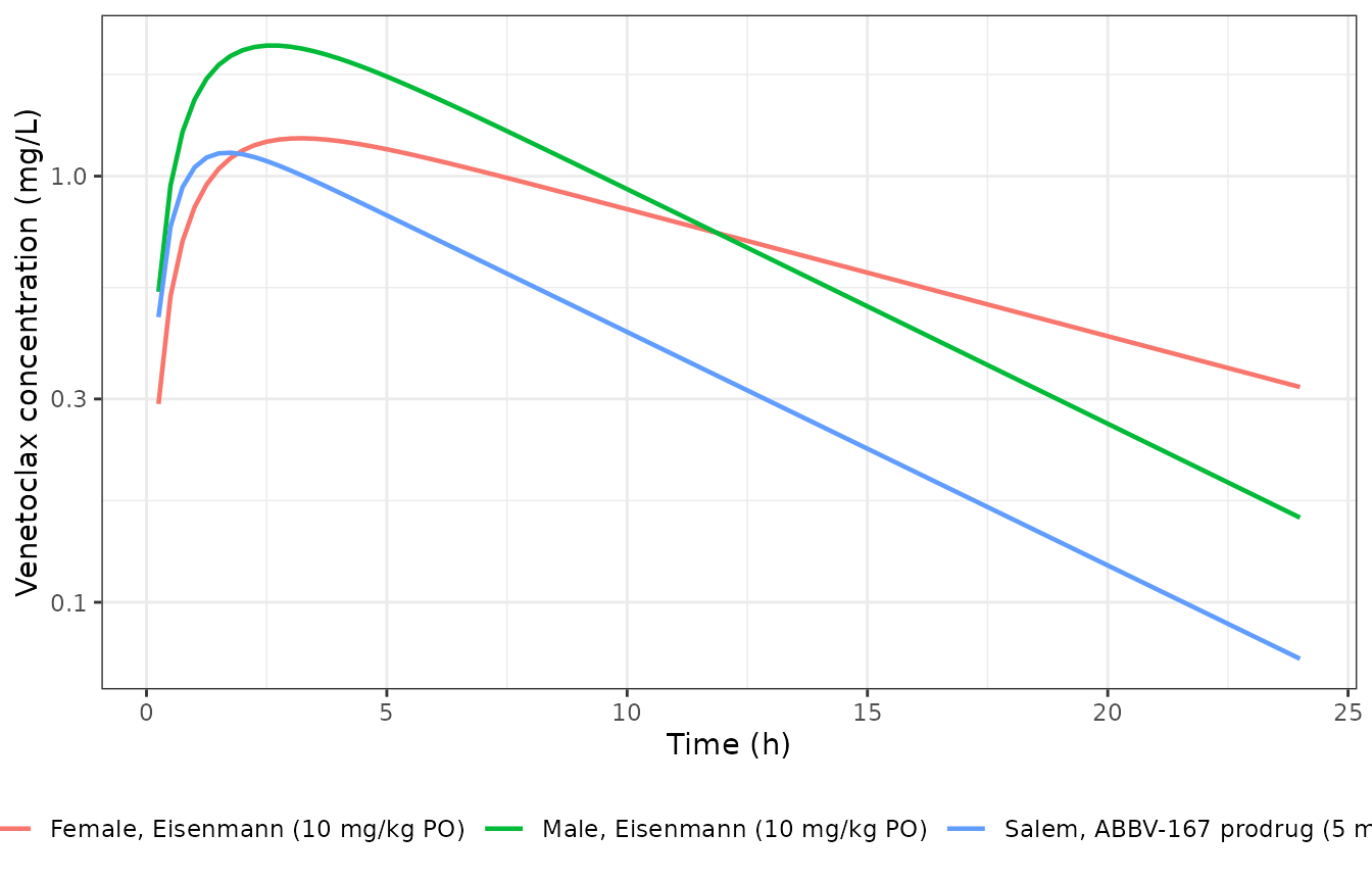
Simulated typical mouse venetoclax profiles for the three fitted cohorts.
Non-compartmental analysis
conc_data <- sim_pk |>
  filter(!is.na(Cc)) |>
  select(id, treatment, time, Cc) |>
  as.data.frame()

dose_data <- cohorts |>
  transmute(id, treatment, amt = dose, time = 0) |>
  as.data.frame()

o_conc <- PKNCA::PKNCAconc(conc_data, Cc ~ time | treatment + id,
                           concu = "mg/L", timeu = "h")
o_dose <- PKNCA::PKNCAdose(dose_data, amt ~ time | treatment + id,
                           doseu = "mg/kg")
o_data <- PKNCA::PKNCAdata(o_conc, o_dose)
o_res <- PKNCA::pk.nca(o_data)

nca_tab <- as.data.frame(o_res) |>
  filter(PPTESTCD %in% c("cmax", "tmax", "auclast", "aucinf.obs", "half.life")) |>
  select(treatment, PPTESTCD, PPORRES) |>
  pivot_wider(names_from = PPTESTCD, values_from = PPORRES) |>
  left_join(cohorts |> select(treatment, dose), by = "treatment") |>
  mutate(cl_derived = dose / aucinf.obs) |>
  select(treatment, cmax, tmax, auclast, aucinf.obs, half.life, cl_derived)

nca_tab |>
  rename(
    Cohort = treatment,
    `Cmax (mg/L)` = cmax,
    `Tmax (h)` = tmax,
    `AUC0-last (mg*h/L)` = auclast,
    `AUC0-inf (mg*h/L)` = aucinf.obs,
    `t1/2 (h)` = half.life,
    `Dose / AUC0-inf (L/h/kg)` = cl_derived
  ) |>
  kable(digits = 3,
caption = "Non-compartmental analysis of the simulated mouse profiles.")| Cohort | Cmax (mg/L) | Tmax (h) | AUC0-last (mg*h/L) | AUC0-inf (mg*h/L) | t1/2 (h) | Dose / AUC0-inf (L/h/kg) |
|---|---|---|---|---|---|---|
| Female, Eisenmann (10 mg/kg PO) | 1.227 | 3.25 | 17.604 | 22.296 | 10.164 | 0.449 |
| Male, Eisenmann (10 mg/kg PO) | 2.025 | 2.50 | 21.012 | 22.267 | 5.504 | 0.449 |
| Salem, ABBV-167 prodrug (5 mg/kg IV) | 1.135 | 1.75 | 10.539 | 11.125 | 5.514 | 0.449 |
sim_pk |>
  group_by(treatment) |>
  summarise(vc = first(vc), cl = first(cl), .groups = "drop") |>
  left_join(nca_tab |> select(treatment, aucinf.obs, half.life), by = "treatment") |>
  transmute(
    Cohort = treatment,
    `t1/2 from NCA (h)` = half.life,
    `ln(2) * V / CL (h)` = log(2) * vc / cl,
    `Dose / AUC0-inf (L/h/kg)` = nca_tab$cl_derived[match(treatment, nca_tab$treatment)],
    `Fitted CL (L/h/kg)` = cl
  ) |>
  kable(digits = 3,
caption = "Internal consistency of the NCA against the fitted structural parameters.")| Cohort | t1/2 from NCA (h) | ln(2) * V / CL (h) | Dose / AUC0-inf (L/h/kg) | Fitted CL (L/h/kg) |
|---|---|---|---|---|
| Female, Eisenmann (10 mg/kg PO) | 10.164 | 10.096 | 0.449 | 0.449 |
| Male, Eisenmann (10 mg/kg PO) | 5.504 | 5.465 | 0.449 | 0.449 |
| Salem, ABBV-167 prodrug (5 mg/kg IV) | 5.514 | 5.495 | 0.449 | 0.449 |
Derippe 2024 reports no NCA metrics of its own, so there is no
published table to compare against; the check available here is internal
consistency, shown above. The terminal half-life recovered by NCA
matches ln(2) * V / CL for each cohort, and
Dose / AUC0-inf recovers the fitted clearance of 0.449
L/h/kg (exactly, since these are noise-free typical-value profiles and
the model is linear). The authors themselves note the terminal half-life
is over-predicted relative to the digitized data, because the Eisenmann
profiles only run to 6 h and were still on a plateau there.
Model 3 – SU-DHL-4 xenograft growth
# Digitized vehicle-control arm (deposit data/mice_SU_DHL4_full.csv), which is
# the arm the Supporting Information 'Control PD modeling' section was fit to.
control_obs <- tibble::tribble(
  ~time, ~tumor_mm3,
      0,   255.87372,
      3,   323.67307,
      5,   484.40190,
      8,   769.78460,
     11,  1099.52760,
     15,  1819.85030
)

tgi_ev <- tibble::tibble(id = 1L, time = seq(0, 21, by = 0.5)) |>
  mutate(evid = 0L, amt = NA_real_, cmt = "tumor_size")

sim_tgi <- rxode2::rxSolve(tgi, tgi_ev, useLinCmt = FALSE) |>
  as.data.frame()

stopifnot(n_ids(sim_tgi) == 1L)

pred <- approx(sim_tgi$time, sim_tgi$tumor_size, xout = control_obs$time)$y

control_obs |>
  mutate(
    Predicted = round(pred, 1),
    `Percent error` = round(100 * (pred - tumor_mm3) / tumor_mm3, 1)
  ) |>
  rename(`Day` = time, `Observed (mm^3)` = tumor_mm3, `Predicted (mm^3)` = Predicted) |>
kable(caption = "Exponential growth model vs the digitized vehicle-control arm.")| Day | Observed (mm^3) | Predicted (mm^3) | Percent error |
|---|---|---|---|
| 0 | 255.8737 | 258.0 | 0.8 |
| 3 | 323.6731 | 382.6 | 18.2 |
| 5 | 484.4019 | 497.4 | 2.7 |
| 8 | 769.7846 | 737.6 | -4.2 |
| 11 | 1099.5276 | 1093.6 | -0.5 |
| 15 | 1819.8503 | 1849.1 | 1.6 |
ggplot(sim_tgi, aes(time, tumor_size)) +
  geom_line(linewidth = 0.8) +
  geom_point(data = control_obs, aes(time, tumor_mm3), size = 2.5) +
  labs(x = "Time (days)", y = expression(paste("Tumor volume (", mm^3, ")"))) +
  theme_bw()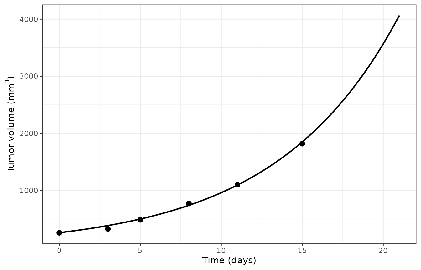
Untreated SU-DHL-4 xenograft growth: model prediction against the digitized control observations.
Five of the six observations are within 5%; the day-3 point is over-predicted by 18%, which is the single largest residual and is consistent with the reported additive residual SD of 24.3 mm^3 being small relative to scatter in a digitized group-mean curve. The overall agreement is the check that settles the unit question raised in the Errata below: read as 1/day the model tracks the data across the whole window, whereas the printed 1/h would imply a 5.3-hour tumor doubling time.
Assumptions and deviations
Errata and source conflicts
1. Tumor growth rate constant units. The Supporting
Information states the exponential growth rate constant is “0.1313
h^-1”. It is per day. Three independent lines of
evidence agree: (a) an ordinary least-squares fit of
log(volume) on day to the deposited control data gives
0.136 1/day with an intercept of 243 mm^3, matching the reported Monolix
estimates of 0.1313 and 258 mm^3; (b) the agent-based model in the same
Supplement consumes the constant as
probability = kgrowth x step with
step = 0.1 days; (c) 0.1313 1/h would be a 5.3-hour
doubling time. The model file encodes 1/day.
2. Clearance units in the mouse PK table. The “Mice
PK modeling” table prints Cl (L/h, RSE %) alongside
V (L/kg). Clearance must be L/h/kg for CL/V to
have units of 1/h; the deposited QSP code computes
Ke_Veneto <- Cl_Veneto / Vd_Veneto directly from these
two numbers, giving 0.127 1/h. The model file encodes L/h/kg.
3. BAX/BAK turnover rate. The Supplement prose says
every BAX/BAK-containing compartment degrades with a “half-life = 22 h”,
which implies 0.0315 1/h. The deposited code – which is what generated
every published result – uses kelimBAXBAK = 0.014 1/h, a
half-life of 49.5 h. The extracted model follows the code. Users wanting
the prose value can override kelimBAXBAK = log(2) / 22.
4. A-1210477 top concentration. The Methods state
A-1210477 was tested at “0, 5, 10, or 20 uM”. Both the deposited assay
dataset (data/data_cell_viability.csv) and the deposited
celltheque column names use 15 uM as the top level. The
vignette and the model documentation use 15 uM.
5. d/dt(Bclxl_BAKa) carries six foreign flux
terms. In the deposited model the BCL-XL:activated-BAK balance
is written as
R37 - R36 - R38 - R40 - R53 - 2*R65 - kelim*Bclxl_BAKa; the
six subtracted terms are the entire right-hand side of
d/dt(BAXma) and have no mechanistic place in a BCL-XL:BAK
complex balance. Every sibling complex (Bcl2_BAKa,
Mcl1_BAKa, Bclxl_BAXma) is written in the
expected R_complex - kelim*state form, so this is almost
certainly a copy-paste artefact. It is not inert:
Bclxl_BAKa feeds back into R37, and hence into
free BCL-XL and activated BAK. Because this is the code that produced
every published figure and every deposited cell-fate record – which the
extracted model reproduces exactly, see the celltheque check above – the
equation is retained verbatim rather than silently corrected. The
structurally intended form would be
d/dt(Bclxl_BAKa) <- R37_complex_Bclxl_BAKa - Bclxl_BAKa * kelimBAXBAK * switchE.
6. Mixed concentration units in the drug-effect
term. The deposited model computes both
Veneto_plasma (mg/L) and
Veneto_plasma_microMolai (uM) but feeds the
mg/L value into Veneto_tumor, which is
then multiplied by k2_Bcl2_I in 1/uM/h. The two differ by
the molar mass factor 868.44/1000 = 0.868. In practice this is absorbed
by the plasma-to-tumor conversion factor, which the authors themselves
describe as carrying “very high uncertainty” (they assume 0.3). Retained
as deposited; noted so a downstream user does not treat
ratioTumor as a purely physiological quantity. The in-vitro
exposures (Bcl2_I0 etc.) are unaffected – they are in uM
throughout.
Assumptions made in this extraction
-
Default virtual cell. The apoptosis model ships the
eight protein levels of virtual cell 4272, the modal cell of
both published three-drug calibrated virtual tumors (11 of 100
cells in SU-DHL-4, 9 of 100 in KARPAS-422). Any other cell can be
supplied through
rxSolve(params = ...). These eight parameters are deliberately not wrapped infixed(): they are the model’s intended degrees of freedom. -
Oligomerisation constants consolidated. The
deposited code assigns
0.0461/0.695to all twelve BAK and twelve BAX oligomerisation steps, re-assigning several of the same names more than once with the same value. These are carried as a single shared pair (kforward_olig/kbackward_olig). Likewise the per-partner dissociation constants, which are identical across every partner of a given antiapoptotic protein, are carried askbackward_Bcl2/_Bclxl/_Mcl1, and the six identical activator-effector constants askforward_act/kbackward_act/k_activation. No numeric value is changed by this consolidation. -
ratioTumordefault. Shipped as 1 (the deposited in-vitro default). The in-vivo simulations in the paper set it to 0.3. -
Mouse PK covariate coefficients are back-calculated
as ratios (3.54/6.54, 3.56/6.54, 1.65/0.856) because the Supplement
prints the resulting parameter per group rather than the coefficient.
The reference group is female, which is the reverse of
the usual nlmixr2lib convention; this follows the paper’s own table
layout. Set
SEXF = 0for Salem-study records – the sex term is switched off there by construction. - No inter-individual variability is encoded anywhere. None of the three models reports an IIV term: the QSP model is deterministic per cell (cell-level heterogeneity is expressed through the virtual-cell population, not through etas), and the mouse PK and tumor growth fits report only residual error. No variance was invented.
- Not extracted: the agent-based model (stochastic and discrete-event, not an ODE system), the PaSM parameter-space-mapping accelerator (a simulation algorithm, not a model), and the VT calibration objective function and its penalty terms (a fitting procedure). The A-1592668 K-PD arm is encoded, but its EC50 is a placeholder the authors chose small enough to force complete MCL-1 shutdown rather than an estimated potency.
- Not modelled: the navitoclax viability curves present in the deposited assay dataset. The paper calibrates on venetoclax and A-1155463 only (80 points per cell line), so no navitoclax parameters exist.
Session information
sessionInfo()
#> R version 4.6.1 (2026-06-24)
#> Platform: x86_64-pc-linux-gnu
#> Running under: Ubuntu 24.04.5 LTS
#>
#> Matrix products: default
#> BLAS:   /usr/lib/x86_64-linux-gnu/openblas-pthread/libblas.so.3
#> LAPACK: /usr/lib/x86_64-linux-gnu/openblas-pthread/libopenblasp-r0.3.26.so;  LAPACK version 3.12.0
#>
#> locale:
#>  [1] LC_CTYPE=C.UTF-8       LC_NUMERIC=C           LC_TIME=C.UTF-8
#>  [4] LC_COLLATE=C.UTF-8     LC_MONETARY=C.UTF-8    LC_MESSAGES=C.UTF-8
#>  [7] LC_PAPER=C.UTF-8       LC_NAME=C              LC_ADDRESS=C
#> [10] LC_TELEPHONE=C         LC_MEASUREMENT=C.UTF-8 LC_IDENTIFICATION=C
#>
#> time zone: UTC
#> tzcode source: system (glibc)
#>
#> attached base packages:
#> [1] stats     graphics  grDevices utils     datasets  methods   base
#>
#> other attached packages:
#> [1] knitr_1.52            ggplot2_4.0.3         tidyr_1.3.2
#> [4] dplyr_1.2.1           PKNCA_0.12.1          rxode2_5.1.8
#> [7] nlmixr2lib_0.3.2.9000
#>
#> loaded via a namespace (and not attached):
#>  [1] gtable_0.3.6        xfun_0.61           bslib_0.12.0
#>  [4] rxode2lincmt_0.1.0  lattice_0.22-9      vctrs_0.7.3
#>  [7] tools_4.6.1         generics_0.1.4      parallel_4.6.1
#> [10] tibble_3.3.1        symengine_0.2.14    pkgconfig_2.0.3
#> [13] data.table_1.18.6.1 checkmate_2.3.4     RColorBrewer_1.1-3
#> [16] S7_0.2.2            desc_1.4.3          lifecycle_1.0.5
#> [19] compiler_4.6.1      farver_2.1.2        textshaping_1.0.5
#> [22] fontawesome_0.5.3   htmltools_0.5.9     sys_3.4.3
#> [25] sass_0.4.10         yaml_2.3.12         pillar_1.11.1
#> [28] pkgdown_2.2.1       crayon_1.5.3        jquerylib_0.1.4
#> [31] whisker_0.4.1       openssl_2.4.2       cachem_1.1.0
#> [34] nlme_3.1-169        tidyselect_1.2.1    digest_0.6.39
#> [37] lotri_1.0.5         purrr_1.2.2         labeling_0.4.3
#> [40] rxode2ll_2.0.18     fastmap_1.2.0       grid_4.6.1
#> [43] cli_3.6.6           dparser_1.3.1-14    magrittr_2.0.5
#> [46] withr_3.0.3         scales_1.4.0        backports_1.5.1
#> [49] rmarkdown_2.32      otel_0.2.0          askpass_1.2.1
#> [52] ragg_1.5.2          memoise_2.0.1       evaluate_1.0.5
#> [55] rex_1.2.2           PreciseSums_0.7     rlang_1.3.0
#> [58] downlit_0.4.5       Rcpp_1.1.2          glue_1.8.1
#> [61] xml2_1.6.0          jsonlite_2.0.0      R6_2.6.1
#> [64] systemfonts_1.3.2   fs_2.1.0